Load Balancing in Downlink LTE Self-Optimizing Networks Andreas Lobinger∗ , Szymon Stefanski† , Thomas Jansen‡ , Irina Balan§ ∗
Nokia Siemens Networks, M¨unchen, Germany,
[email protected] Nokia Siemens Networks, Wrocław, Poland,
[email protected] ‡ Technical University of Braunschweig, Braunschweig, Germany,
[email protected] § Interdisciplinary Institute for Broadband Technology, Ghent, Belgium,
[email protected] †
Abstract—In this paper we present system level simulation results of a self-optimizing load balancing algorithm in a longterm-evolution (LTE) mobile communication system. Based on previous work [2][1], we evaluate the network performance of this algorithm that requires the load of a cell as input and controls the handover parameters. We compare the results for different simulation setups: for a basic, regular network setup, a non-regular grid with different cell sizes and also for a realistic scenario based on measurements and realistic traffic setup.
•
I. I NTRODUCTION
•
In existing networks, parameters are manually adjusted to obtain a high level of network operational performance. In LTE the concept of self-optimizing networks (SON) is introduced, where the parameter tuning is done automatically based on measurements. A challenge is to deliver additional performance gain further improving network efficiency. The use of load-balancing (LB), which belongs to the group of suggested SON functions for LTE network operations, is meant to deliver this extra gain in terms of network performance. For LB this is achieved by adjusting the network control parameters in such a way that overloaded cells can offload the excess traffic to lowloaded adjacent cells, whenever available. In a live network high load fluctuations occurs and they are usually accounted for by overdimensioning the network during planning phase. A SON enabled network, where the proposed SON algorithm monitors the network and reacts to these peaks in load, can achieve better performance by distributing the load among neighbouring cells [10]. The load balancing algorithm aims at finding the optimum handover (HO) offset value between the overloaded cell and a possible target cell. This optimised offset value will assure that the users that are handed over to the target cell will not be returned to the source cell and thus the load in the current cell is diminished. Simulations were conducted for synthetic regular hexagonal and non regular network layout as well as a realistic network scenario. The work has been carried out in the EU FP7 SOCRATES project [1]. II. D EFINITIONS AND M ETRIC In [2] a mathematical framework for SON investigations on the downlink is defined. The main parts for this mathematical framework are recalled below:
• •
•
A network layout by network nodes, eNodeB(s) (eNB), defining a cell c at the position p!c . A user u located at a position !qu . In dynamic simulation the user positions can be evolve over simulation time. A connection function X(u), following that a user u is served by cell c = X(u) with the constraint (according to the definition of LTE) that every user is connected exactly to a single cell. A pathloss mapping L, LX(u) (!qu ) defined by the positions of user u relative to a cell c, c = X(u). The pathloss mapping takes all position-dependent channel model effects into account, which are: distance-dependent pathloss, shadowing and angle-dependent antenna patterns. A cell load ρc , which defines the ratio of used resources in LTE physical resource blocks (PRBs) to all available resources in a given cell.
With the above framework and two additional terms i.e. N as thermal noise and Pc as transmit power for a cell, we can now define and evaluate for every user, in every time-step a user specific signal to noise and interference ratio, SIN Ru . SIN Ru =
N+
!
Pc · LX(u) (!qu ) . qu ) c!=X(u) ρc · Pc · Lc (!
(1)
The evaluation complexity is reduced by the selection of a single service definition for all users, a constant bit rate (CBR) service. The CBR assumption used further on is 512kBit/s. A. Load and throughput mapping We assume that the best modulation coding scheme (MCS) is used for a given SINR and the highest data rate R(SIN R) is achievable, this can be represented by Shannon formula. R(SIN Ru ) = log2 (1 + SIN Ru )
(2)
However for better approximation to realistic MCS, the mapping function is scaled by a factor 0.6 and is bounded by maximum available bitrate (4.4 bps/Hz) and minimum required SINR (-6.5 dB), a detailed description of which can be found in [4]. Based on the achievable throughput at a given SINR, the demanded data rate D and the transmission bandwidth BW of one PRB (PRB bandwidth in LTE system is 180kHz),
data rate
required PRBs for 512 kb/s
5
18 16 14 12
3
10 8
2
6
required PRBs N
data rate R [bps/Hz]
4
4
1
2 0
0 -7
-5
-3
-1
1
3
5
7
9
11
13
15
17
19
21
23
25
SINR [dB]
TeNB. This issue should be controlled by admission and congestion control mechanisms in the TeNB. When the admission and congestion control mechanisms reject LB HO requests, there will be a significant increase in signaling overhead if the requests are repeated. We propose a prediction method to adress this for the load required at TeNB side, based on SINR estimation after LB HO, taking into account UE measurements like the reference signal received power (RSRP) and received signal strength indicator (RSSI). For simplification we do not consider additional factors related to the current load at SeNB and TeNB which may have an impact on SINR. Signal received by user u from cell c we can write as:
Fig. 1. Required PRBs for transmission of 512 kbps as a function of SINR.
the amount of required PRBs N can be obtained from the following: Du Nu = (3) R(SIN Ru ) · BW Figure 1 presents the relationship between SINR, throughput and required resources in DL transmission. B. Virtual load and unsatisfied users metric In this document we investigate scenarios with different load distributions including user u concentrations to overload the serving cell. The overload situation occurs when the total required number of PRBs Nu may exceed the amount of the total available resources in one cell MP RB . Thus we introduce the virtual cell load, ρ"c which can be expressed as the sum of the required resources of all users u connected to the cell c by the connection function X(u) which gives the serving cell c for user u # 1 ρ"c = · Nu . (4) MP RB u|X(u)=c
This metric allows us to exceed 100% of cell load (ρ"c >1) and such situations indicate a scale of overload in cell c. In overloaded cells part of the users can not be served with the required service quality and we call them as unsatisfied. The total number of unsatisfied users in the whole network (users being a sum of unsatisfied users in all cells, where number of users in cell c is represented by Mc ) can be written as: $ $ %% # 1 z= max 0, Mc · 1 − (5) ρ"c ∀c
Detailed explanation of the virtual load concept and unsatisfied users metrics can be found in [2]. C. Load estimation
Load balancing is achieved by handing over users from the overloaded cells to those adjacent cells which are able to accommodate additional load. After HO, the user’s SINR condition at cell served by target eNB (TeNB) as well as generated load is different than in previous cell served by serving eNB (SeNB). The load transferred during LB operation should not exceed the capacity reported as available by the
Sc = Pc · Lc (!qu )
(6)
Before LB HO the user u1 is connected to the SeNB, SeN B = X(u1 ) with the strongest received RSRP signal (signal S1 in Figure 2 a). The RSRP signal from TeNB (S2 in Figure 2a) is a component of total interference as well as signals originated from other eNBs (represented by I in Figure 2a). After HO of user u1 to TeNB, received signal S1 from the previously serving SeNB now contributes to the interference signal at u1 whereas signal S2 from TeNB is the wanted signal (see Figure 2b). a)
I± interference from
othereN B
SeN B S1
S2
u3
TeN B
u1 u2
I± interference from
b) SeN B S1
othereN B
S2 u3
TeN B
u1 u2
Fig. 2.
Signals received by UE a) before HO, b) after HO
We assume that during the time of HO execution, the user’s u1 position !qu1 does not change significantly and hence we also assume no changes of received signal power by the user u1 . We can extract signals S1 and S2 from the interference part of SIN RSeN B and SIN RT eN B equations and after combining them, this relation can be written as follows:
SIN Ru1 ,T eN B =
S2 . S1 + S1 − S2 SIN Ru1 ,SeN B
(7)
III. L OAD BALANCING ALGORITHM
Algorithm 1 HO offset based LB algorithm Require: List L of potential Target eNB (TeNB) for LB HO 1. collect measurements from user:; RSRP to potential TeNB, 2. group users corresponding to the best TeNB for LB HO (criterion is the difference between SeNB and TeNB measured signal quality), 3. obtain information from TeNB on available resources, 4. estimate a number of required PRBs after LB HO for each user in the LB HO group, 5. T ⇐ 0 6. while ρSeN B > ρT hld,SeN B ∧ T < Tmax do 7. i⇐1 8. T ⇐ T + step 9. L ⇐ sort (TeNB according to number of users allowed to LB HO with given T, descending order ) 10. while ρSeN B > ρT hld,SeN B ∧ i ≤ size(L) do 11. C ⇐ L(i) {take next cell from list} 12. estimate ρ"c after HO for given T 13. if ρ"c < ρT hld,C then 14. ρSeN B ⇐ ρSeN B − ρSeN B,T {update load in overloaded cell by substract handed over load} 15. TC,u ⇐ T 16. end if 17. i⇐i+1 18. end while 19. end while 20. adjust HO offsets TC
800
1500
600
1000
400
500 Y [m]
200 Y [m]
In this investigation we are using the parameter “cell specific offset” to force users to handover from the SeNB to a TeNB. It is important to set this parameter carefully, so as not to exceed the acceptable load at TeNB after the LB HO procedure. The main goal of the presented Algorithm 1 is to find the optimum HO offset that allows the maximum number of users to change cell without any rejections by admission control mechanism at TeNB side. Before applying the LB procedure, the SeNB needs to create a list of potential targets for HO, collect measurement reports from the served UEs as well as to collect the available resources reports from neighbouring cells. These preparation actions are included in steps 1 - 5 of Algorithm 1. For each adjusted values of HO offset T , SeNB sorts the list of the potential TeNB with respect to the number of possible LB HOs. Subsequently, for given HO offset T and cell C from the list L a load after HO, ρ"c , is estimated. If the predicted load ρ"c does not exceed acceptable level ρT hld at TeNB, HO offset to this cell is adjusted to the T value and virtual load at SeNB ρSeN B is reduced by the amount generated by the users handed over with this offset. Algorithm works until load ρSeN B at SeNB is higher than accepted level ρT hld,SeN B and HO offset is below the maximum alowed value and neighbour cells are able to accommodate additional load.
2000
1000
0
0
-200
-500
-400
Base Station -1000 antenna orientation hotspot -1500 users in hotspot equal distributed users -2000
-600 -800 -1000 -1000
-500
0
500
1000
-2000
-1000
X [m]
Fig. 3.
0
1000
X [m]
Regular and non-regular simulation scenarios with hotspot path
IV. S IMULATION S CENARIOS As already mentioned a standard LTE DL system of 10MHz bandwidth is used with the simulation assumptions in the LTE 3GPP definitions [7]. For both the synthetic and real scenario a simulation time-step of 500ms have been used. So all internal signals, evaluations and updates are carried out with averaging over this 500ms step. Also the LB algorithm is called in every time-step. A. Synthetic scenario Following the standard simulation assumptions a simulation setup with 19 sites in a regular hexagonal grid, 3 sectors per site and 57 cells are defined. Additionally, a non-regular grid with 12 sites, 3 sectors per site and 36 cells is used as comparison taking real network effects like different cell sizes, number of neighbor cells and interference situations into account. For employing localized higher load in the system a simulation scenario is used here with a setup of background load in all cells with a low number of users -so they are satisfied in any position of the network- and an additional hotspot in which new, additional users are dropped over time. The hotspot area is moved over time on a path through the network as depicted in Figure 3. The channel model is defined in closed form [7], so the pathloss mapping L is continuos. The movement of the users (whether background or dropped in the hotspot) is a constant velocity and random waypoint model. B. Real scenario The realistic reference scenario in the SOCRATES project is an LTE network based on the real layout of the existing 2G and 3G macro networks provided by a network operator (see [8] for more details). The scenario data includes the following information: Network configuration, Pathloss data, Clutter data, Heigth data, Traffic data, Mobility data. An area of 72 km x 37 km is selected. The resulting network comprising of 103 sites and 309 cells is shown partly in Figure 4. For a smaller area of 1.5 km x 1.5 km within the realistic scenario the detailed microscopic mobility model SUMO (Simulation of Urban MObility) is used [11] to introduce relevant user mobility. The mobile users in this mobility model are cars and thus travel along streets. The
Fig. 5.
mobility model incorporates traffic lights, multiple lanes, user acceleration and braking, queueing in front of barricades and overtaking of slower cars. In order to generate an overload in the scenario a moving hotspot is defined by a bus with a set of users moving together along a road. The distribution of additional static users is based on traffic maps provided by the same operator. Based on operator measurements and path predictions using a ray-tracer a pathloss mapping L is now available for background users (static + mobile) and the users in the bus (hotspot). For this pathloss mapping only the 30 most significant cells -including both the connected cell and the interfering cells- are taken into account. In Figure 5 the path of the bus is shown in more detail. Gray shapes make an image of the city streets and magenta lines determine the theoretical cells marked by numbers. Base stations and antennas orientations are shown in the same way as on Figure 3. Bus route is tagged by the brown colour. Circle markers with the letters correspond to the points of HO of more than 50% of the users in bus. Starting from the cell a are handovered to cell #104 #105; users in bus at point % a → 104. Following sequence describe the it is writen as: % HO scheme of the bus users during the 10 min simulation of a → 104; % b → 105; % c → 103; % d → 50; reference case: % e → 103; % f → 50; % g → 99; % h → 50; % i → 15; % j → 97; % k → 15; % l → 144. % V. R ESULTS
A. Synthetic Scenarios In Figures 6 and 7 timeline of the z-metric for each simulation scenario with a reference system (red curve) versus loadbalancing (green curve) are depicted. The operating point here -in both scenarios- is 5 users per cell in background (equally dropped) and 40 users dropped in hotspot. The performance of
the load-balancing is -as expected- dependent on the hotspot position and on the users positions within the hotspot. The averaged unsatisfied users metric z is depicted as horizontal line. In table I some more operating points and the average results are shown as overview. unsatisfied users z
Realistic Scenario, area with basestation positions
21 18 15 12 _ 9 z = 7.68 6 _ 3 z = 2.03 0 0 100
Fig. 6.
unsatisfied users z
Fig. 4.
Realistic Scenario, hotspot (bus) path
200
300 time [s]
400
Load Balancig
500
600
Load Balancing performance over time, regular network
21 18 15 _ 12 z = 9.78 9 _ 6 z = 4.47 3 0 0 100
Fig. 7.
reference system
reference system
200
300 time [s]
400
Load Balancig
500
600
Load Balancing performance over time, non regular network
B. Real Scenario In Figure 8 a timeline of the z-metric for the real simulation scenario with a reference system (red curve) versus loadbalancing (green curve) is depicted. As descriped in IV-B part of the users move together on a bus along a street. Different than the operating point chosen for the synthetic scenarios here a significant background load with 80 static and 80 slow
TABLE I S YNTHETIC SCENARIO , AVERAGE NUMBER OF UNSATISFIED USERS z¯ load-balancing
regular
non-reg.
regular
non-reg.
2.8 7.7 13.6 22.0
3.2 9.8 16.8 23.1
0.3 2.0 6.4 15.5
0.7 4.5 10.6 17.4
virtual load
scenario
users in hotspot 30 40 50 60
z¯ reference system
Reference
10
cell #103 cell #104 cell #105
8 6 4 2 0 0
25
a
50
unsatisfied users z
120 100 80 60 40 20 0 0
reference system
_ z = 63.4
a
c b
Fig. 8.
_ z = 47
e
d
100
Load Balancig
200
f
300 time [s]
g
j l k h i 400
500
600
Load Balancing performance over time, realistic scenario
TABLE II R EALISTIC SCENARIO , AVERAGE NUMBER OF UNSATISFIED USERS users in bus 20 30 40 50 60
z¯ reference system 47.0 53.8 63.4 74.3 86.6
z¯ load-balancing 30.6 37.8 47.0 58.8 68.2
VI. C ONCLUSION AND O UTLOOK In this paper we describe a simulation campaign of a load-balancing algorithm. The algorithm evaluates the load condition in a cell and the neighbouring cells and estimates the impact of changing the HO parameters in order to improve the overall performance of the network. We propose a method for load estimation after HO would occur, which is based on SINR prediction and utilise UE measurements. The efficiency of LB algorithm was checked in simulation of synthetic networks layout as well as for a part of real network in which load situation changes dynamically. An overall load-balancing gain is visible in all simulated scenarios in the provided timelines and tables; leading to the general conclusion that the average number of satisfied users can be improved with load-balancing. The possible gain depends on the local load situation and the available capacity
virtual load
10
moving users is used. In Figure 9 we can observe load (virtual load as defined in Equation 4) variations during the first 300s of the simulation. The markers in Figures 8 and 9 correspond to Figure 5 and the description in section IV-B. Comparing reference and load-balancing timelines we can see that the load-balancing algorithm can redistribute load to neighboring cells which significantly reduces overload in whole observed period. In table II more operating operating points and average results are shown as overview.
b c
d
e
75 100 125 150 175 200 225 250 275 300 time [s] Load Balancing cell #103 cell #104 cell #105
8 6 4 2 0 0
Fig. 9.
25
a
50
b c
d
e
75 100 125 150 175 200 225 250 275 300 time [s]
Virtual load ρ " over time in seperate cells, realistic scenario
in the neighbouring cells. The algorithm relies on capacity available in the neighbouring cells around overloaded cells and the proposed load-balancing algorithm can redistribute the load by changing the HO parameters; If no capacity is available around, the network parameters and so the network performance are left unchanged. R EFERENCES [1] SOCRATES, Self-optimisation and self-configuration in wireless networks, European Research Project, http://www.fp7-socrates.eu. [2] I. Viering, M. D¨ottling, A. Lobinger, A mathematical perspective of self-optimizing wireless networks, IEEE International Conference on Communications 2009 (ICC), Dresden, Germany, May 2009. [3] 3GPP, Self-configuring and self-optimizing network use cases and solutions, Technical Report TR 36.902, available at http://www.3gpp.org. [4] 3GPP, 3rd Generation Partnership Project;Technical Specification Group Radio Access Network;Evolved Universal Terrestrial Radio Access (EUTRA);Radio Frequency (RF) system scenarios (Release 8), Technical Report TR 36.942, available at http://www.3gpp.org. [5] M. Amirijoo, R. Litjens, K. Spaey, M. D¨ottling, T. Jansen, N. Scully, and U. T¨urke, ”Use Cases, Requirements and Assessment Criteria for Future Self-Organising Radio Access Networks,” Proc. 3rd Intl. Workshop on Self-Organizing Systems, IWSOS 08, Vienna, Austria, December 10-12, 2008. [6] Next Generation Mobile Networks, Use Cases related to Self Organising Network, Overall Description, available at http://www.ngmn.org. [7] 3GPP, Physical Layer Aspects for evolved Universal Terrestrial Radio Access (E-UTRAN), Technical Report TR 25.814, available at http://www.3gpp.org. [8] N. Scully, J. Turk, R. Litjens, U. T¨urke, M. Amirijoo, T. Jansen, L. Schmelz, ”Review of use cases and framework II”, Deliverable 2.6 EUProjekt SOCRATES (FP7-2007-INFSO-ICT-216284), March, 2009 [9] 3GPP, Evolved Universal Terrestrial Radio Access Network (E-UTRAN); X2 Application Protocol (X2AP), Technical Specification TS 36.423, available at http://www.3gpp.org. [10] U. T¨urke, and M. Koonert, ”Advanced site configuration techniques for automatic UMTS radio network design,” Proc. Vehicular Technology conference VTC 2005 Spring, vol. 3, pp. 1960-1964, Stockholm, Sweden, May 2005. [11] H. Schumacher, M. Schack and T. K¨urner, ”Coupling of Simulators for the Investigation of Car-to-X Communication Aspects” 7th COST2100 Management Committee Meeting, TD(09)773, Braunschweig, Germany, February 2009.