Nov 18, 2016 - Chicago, Room 322 SEO, 851 S. Morgan Street, Chicago, Illinois, 60607, ... Keywords: adaption, automatic, computational complexity, function ...... staunch scientific software, J. Open Research Software 2 (2014) 1â7. doi:10.
Local Adaption for Approximation and Minimization of Univariate Functions
arXiv:1606.02766v1 [math.NA] 8 Jun 2016
Sou-Cheng T. Choi, Yuhan Ding, Fred J. Hickernell Department of Applied Mathematics, Illinois Institute of Technology, RE 208, 10 West 32nd Street, Chicago, Illinois, 60616, USA
Xin Tong Department of Mathematics, Statistics, and Computer Science, University of Illinois at Chicago, Room 322 SEO, 851 S. Morgan Street, Chicago, Illinois, 60607, USA
Abstract Most commonly known adaptive algorithms for function approximation and minimization lack theoretical guarantees. Our new locally adaptive algorithms are guaranteed to provide approximants that satisfy a user-specified absolute error tolerance for a cone, C, of non-spiky functions in the Sobolev space W 2,∞ . Our algorithms automatically determine where to sample the function—sampling more densely where the second derivative is larger. The computational cost of our algorithm for approximating a univariate function on a bounded interval �q � with L∞ -error not greater than ε is essentially O kf 00 k 1 /ε , which is the 2
same order as that of the best function approximation algorithm for functions in C. The computational cost of our global minimization algorithm is no worse than that for function approximation and can be substantially smaller if the function significantly exceeds its minimum value over much of its domain. Our algorithms have been implemented in our Guaranteed Automatic Integration Library. Numerical examples are presented to illustrate the performance of our algorithms. Keywords: adaption, automatic, computational complexity, function approximation, function recovery, minimization, optimization 2010 MSC: 65D05, 65D07, 65K05, 68Q25
Preprint submitted to Journal of Complexity
June 10, 2016
1. Introduction The goal of this article is to solve univariate function approximation and global minimization problems by locally adaptive algorithms. For some suitable set, C, of continuous, real-valued functions defined on a finite interval [a, b], we construct algorithms A : (C, (0, ∞)) → L∞ [a, b] and M : (C, (0, ∞)) → R such that for any f ∈ C and any error tolerance ε > 0, kf − A(f, ε)k ≤ ε,
(APP)
0 ≤ M (f, ε) − min f (x) ≤ ε.
(MIN)
a≤x≤b
Here, k·k denotes the L∞ -norm on [a, b]. The algorithms A and M depend only on function values. These algorithms choose their data sites in the domain adaptively, with each new site depending on the function data already obtained. Each algorithm automatically determines when to stop sampling and return the correct answer. These algorithms sample more densely where needed, i.e., they are locally adaptive. Adaptive algorithms relieve the user of having to specify the number of samples required. Only the desired error tolerance is needed. Existing adaptive numerical algorithms for function approximation, such as the MATLAB toolbox Chebfun [7], are successful for some f , but fail for other f . No theory explains for which f Chebfun succeeds. A corresponding situation exists for minimization algorithms, such as min in Chebfun or MATLAB’s built-in fminbnd [17]. Our aim is to provide practical algorithms for both (APP) and (MIN) with theoretical justification. Here we accomplish the following: • The set C for which our algorithms succeed is defined in Section 2.2 to be a cone in W 2,∞ , the Sobolev space of functions whose second-order derivatives have finite sup-norms. Because any algorithm can be fooled by a sufficiently spiky function, this C is defined to exclude functions that are too spiky. The parameters that define C may be chosen to reflect the user’s desire for robustness. We construct a data-based upper bound on
2
kf 00 k[α,β] in (14) in terms of second-order divided differences. This leads to a data-based upper bound on the error of the linear spline in (15). • Algorithms A and M are constructed in Sections 3.1 and 4.1 to solve problems (APP) and (MIN), respectively. These algorithms are based on linear splines. Guarantees of success are provided by Theorems 1 and 5. • The upper bound on the computational cost of Algorithm A is derived �q � in Theorem 2 in Section 3.2, and is essentially O kf 00 k 1 /ε (see (22)). 2 �1/p Rb p 1 Here, k·k 1 denotes the L 2 -quasi-norm: kf kp := a |f | dx ,0 1, h ≤ b − a.
(6)
The set C is a cone because f ∈ C =⇒ cf ∈ C for all real c. Cones of functions are key to the theoretically justified adaptive algorithms in [4], [6], and [18]. A function f with f 00 (α) = f 00 (β) = {0} 6= f 00 ((α + β)/2) may lie inside C only if β − α > 2h. Thus, f 00 cannot have zeros too close to each other. Except near the endpoints of the interval, the definition of C uses values of f 00 on both sides of x to bound max |f 00 (x)|. This allows C to include functions with step discontinuities in their second derivatives, provided that these discontinuities do not occur too close to each other or too close to the ends of the interval. We provide examples of functions lying outside C and similar functions lying inside C. Consider the following two functions defined on [−1, 1] whose second derivatives oscillate wildly near 0:
f100 (x) =
f1 (x) = x4 sin(1/x), (12x2 − 1) sin(1/x) − 6x cos(1/x),
x 6= 0
[−1, 1],
x = 0, f200 (x) = 20 + f100 (x).
f2 (x) = 10x2 + f1 (x),
These functions are plotted in Figure 1. Because the f100 (x) takes on both signs for x arbitrarily close to 0 and on either side of 0, it follows that m(f1 , −h− , 0) = 7
1.5
f1 (x) f2 (x)
10
×10−7 f1 (x)
1
8
0.5
6
0
4
-0.5
2 -1
0 -1
-0.5
0
0.5
-1.5 -0.02
1
-0.01
x
0
0.01
0.02
0.01
0.02
x ×10−3
25
f2 (x)
4
20
3
f1′′ (x) f2′′ (x)
15
2
10 5
1
0
0
-5 -1
-0.5
0
0.5
-0.02
1
-0.01
0
x
x
Figure 1: The examples f1 and f2 and their second derivatives. Note that f200 (x) = f100 (x)+20. This figure is reproducible by TraubMemorial.m in GAIL.
m(f1 , 0, h+ ) = 0 for all h± ∈ [0, 1]. However, max |f100 (0)| = 1, so f1 cannot lie inside C no matter how h and C are defined. On the other hand, m(f2 , α, β) ≥ 13.5 for all −1 ≤ α < β ≤ 1, and max |f200 (x)| ≤ 27 for all x ∈ [−1, 1], so f2 ∈ C if C(0) ≥ 2. Now consider the following hump-shaped function defined on [−1, 1], whose second derivative has jump discontinuities: 1 h 2 4δ + (x − c)2 + (x − c − δ) |x − c − δ| 2δ 2 i f3 (x) = −(x − c + δ) |x − c + δ| , |x − c| ≤ 2δ, 0, otherwise,
8
(7)
30 f3′′ (x)
f3 (x)
1
20
0.8
10
0.6
0
0.4
-10
0.2
-20
0 -0.2 -1
-0.5
0
0.5
-30 -1
1
-0.5
0
0.5
1
x
x
Figure 2: The example f3 with −c = δ = 0.2 and its piecewise constant second derivative. This figure is reproducible by TraubMemorial.m in GAIL.
1 [1 + sign(x − c − δ) − sign(x − c + δ), |x − c| ≤ 2δ, 2 00 f3 (x) = δ 0, otherwise. Here c and δ are parameters satisfying −1 ≤ c − 2δ < c + 2δ ≤ 1. This function and its second derivative are shown in Figure 2 for −c = δ = 0.2. If the hump is wide enough, i.e., δ ≥ 2h, then f3 ∈ C for any choice of C : [0, b−a] → [1, ∞). We see this by examining two cases. For all x ∈ [c−2δ, c+2δ] and all h ∈ ]0, h[ ⊆ ]0, δ/2[, let x− = max(a, x − h) and x+ = min(x + h, b). Then m(f3 , x− , x) = m(f3 , x, x+ ) =
sup |f300 (x)| = δ −2 .
−1≤x≤1
For x ∈ [−1, 1] \ [c − 2δ, c + 2δ] we note that f300 (x) = 0. Thus, the definition of the cone is satisfied. However, if the hump is too narrow, i.e., δ < 2h, then regardless of how C is defined, for x = c − 3δ/2 with δ/2 < h < h, C(h)m(f3 , x − h, x) = C(h)m(f3 , x, x + h) = 0 < |f300 (x)| = δ −2 . This violates the definition of C. For δ < 2h the function f3 is too spiky to lie in the cone C. This example illustrates how the choice of h influences the width of a spiky function that may or may not lie in C. The above examples of functions outside C have discontinuous second-order derivatives. If a function has sufficient smoothness and the higher order deriva9
tives are nicely behaved in a certain sense, then we can be sure that this function lies in C. If f ∈ C 3 [a, b] and for all x ∈ [a, b], the following conditions holds: � � |f 00 (x)| 1 000 kf k[min(a,x−h),max(x+h,b)] ≤ 1− ∀h ∈ [0, h], (8) h C(h) then one must have f ∈ C. Using a Taylor expansion it follows that. m(f, min(a, x − h), max(x + h, b)) = inf |f 00 (] min(a, x − h), max(x + h, b)[)| ≥ |f 00 (x)| − kf 000 k[min(a,x−h),max(x+h,b)] h � � 1 00 00 ≥ |f (x)| − |f (x)| 1 − C(h) 00 |f (x)| ≥ ∀x ∈ [a, b], h ∈ [0, h]. C(h) Thus, f ∈ C by the definition of the cone in (5). Sufficient condition (8) fails if f 00 (x) = 0 for some x. For x ∈]a + h, b − h[ one may replace (8) by an alternative sufficient condition if f ∈ C 4 [a, b]: max
|f 0000 (t)| ≤
0≤s(t−x)≤h
2 |f 00 (x)| h2
� 1−
1 C(h)
� +
2 |f 000 (x)| h
∀h ∈ [0, h], s = sign(f 00 (x)f 000 (x)). (9) Note that here s depends on x. For a particular x, suppose that s = +1. Then it follows by a Taylor expansion that m(f, x, x + h) = inf |f 00 (]x, x + h[)| � � kf 0000 k[x,x+h] (t − x)2 00 000 ≥ inf |f (x)| + |f (x)| (t − x) − x