Nov 5, 1997 - ac1. ¯. Ïϵλγ5. â. Dλ Ï +. 1. 2 ac2âµ( ¯ Ïγ5Ï) ,. (26). â¢tµν = ¯ÏϵνÏ. ( ¯. ÏϵνÏ)imp. = (1 + abm) ¯ÏÏÂµÎ½Ï + i. 1. 2. ac1ǫµνλÏ. ¯ ÏÎ³Ï Î³5. â.
UL-NTZ 37/97 HUB-EP-97/75 DESY 97-216
Local bilinear operators on the lattice and their perturbative renormalisation including O(a) effects
arXiv:hep-lat/9711007v1 5 Nov 1997
S. Capitani1, M. G¨ockeler2, R. Horsley3, H. Perlt4, P. Rakow5, G. Schierholz1,5, A. Schiller4∗ 1 2 3
DESY-Theory Group, Notkestraße 85, D-22607 Hamburg, Germany
Universit¨ at Regensburg, Institut f¨ ur Theoretische Physik, D-93040 Regensburg, Germany Humboldt-Universit¨ at, Institut f¨ ur Physik, Invalidenstraße 110, D-10115 Berlin, Germany 4
Universit¨ at Leipzig, Institut f¨ ur Theoretische Physik and NTZ, Augustusplatz 10-11, D-04109 Leipzig, Germany
5
DESY-I f H Zeuthen, Platanenallee 6, D-15738 Zeuthen, Germany
November 5, 1997 Abstract Some basic concepts are discussed to derive renormalisation factors of local lattice operators relevant to deep inelastic structure functions and to other measurable quantities. These Z factors can be used to relate matrix elements measured by lattice techniques to their continuum counterparts. We discuss the O(a) improvement of point and one–link lattice quark operators. Suitable bases of improved operators are derived. Tadpole improvement is applied to get more reliable perturbative results.
1
Introduction and some basic definitions of DIS and OPE
In deep inelastic lepton scattering (DIS, see e.g. [1]) (with 4–momenta k and k ′ ) on hadron (p with p2 = M 2 ) the inclusive differential cross section for eP → e′ X in the hadron rest frame is given by d3 σ e4 = y lµν (k, q, sl ) Wµν (p, q)λλ (1) 2 4 dx dy dφ 16π Q with the standard notations x=
Q2 , 2p · q
y=
p·q , p·k
(2)
q = k − k ′ (with −q 2 = Q2 ) is the momentum transfer in the scattering process, φ the azimuthal scattering angle of the outgoing lepton, sl (with s2l = −m2l ) the initial lepton polarisation vector and λ denotes the initial hadron polarisation (±1/2 for spin 1/2 target). All information about ∗
Talk given by A. Schiller at 2nd SPIN Workshop, Zeuthen, September 1-5, 1997
1
the cross section is contained in the leptonic and hadronic tensors lµν and Wµν . While lµν is known, the hadronic tensor µν
W (p, q)λ′ λ
1 Z 4 iq·x d x e hp, λ′ |[j µ (x), j ν (0)]|p, λi = 4π
(3)
with the electromagnetic hadronic currents j µ (x) contains the strong interaction effects which are not completely accessible to perturbative QCD. The most general hadronic tensor for polarised DIS from spin 1/2 targets is usually written in the form qµ qν + 2 q
!
p·q Wµν (p, q, s) = F1 −gµν pµ − 2 qµ q ! ρ q s·q σ σ + iǫµνρσ (g1 + g2 )s − g2 p . p·q p·q F2 + p·q
!
p·q pν − 2 qν q
!
(4)
Here F1,2 and g1,2 are the structure functions and sµ the polarisation vector of the nucleon with s2 = −M 2 . In a parton model interpretation the structure functions F1,2 contain information about the overall density of quarks (and gluons) in the nucleon and g1 probes the distribution of quarks of given helicity in a longitudinally polarised nucleon (Qi is the quark charge, q± (x)(q ± (x)) denotes the distribution function of quark (antiquark) with momentum fraction x and helicity parallel/antiparallel to its parent nucleon) F1 (x, Q2 ) =
X i
2
F2 (x, Q ) =
X i
2
g1 (x, Q ) =
X i
� Q2i � q+ (x) + q− (x) + q+ (x) + q − (x) , 2 �
�
Q2i x q+ (x) + q− (x) + q + (x) + q − (x) ,
(5)
� Q2i � q+ (x) − q− (x) + q + (x) − q − (x) . 2
The structure function g2 has no simple interpretation in the parton model. One can derive sum rules (moments) for the structure functions directly from QCD using the operator product expansion (OPE). The starting point is the time–ordered product of two hadronic currents Z tµν = i d4 z eiq·z T (jµ (z) jν (0)) (6) the matrix element of which gives the well–known Compton amplitude. This amplitude is related to the hadronic tensor Wµν via the optical theorem 2πWµν (p, q)λ′ λ = Im hp, λ′ |tµν |p, λi .
(7)
To calculate the Compton amplitude in QCD one relies on OPE which allows to write the product of two local operators Oa (z) and Ob (0) for vanishing distance z as an expansion in local operators. In the Fourier transform version of OPE one has lim q→∞
Z
d4 z eiq·z Oa (z)Ob (0) =
X
cabd (q)Od (0) .
(8)
d
The Wilson coefficients cabd (q) (in general singular at q → ∞) are independent of the matrix elements, provided q is much larger than the characteristic momentum in any of the external states. 2
The local operators in OPE for QCD are quark and gluon operators with arbitrary dimension d and spin n. It can be shown that the contribution of any operator to lµν Wµν is of the order µ1 ...µn cµ1 ...µn Od,n
Q2 M2
−n
∝x
!(2−t)/2
(9)
with the twist introduced as t = d − n. Therefore, the most important operators in OPE at Q2 → ∞ are those with twist two contributing to F1,2 and g1 . The structure function g2 involves twist three operators allowing a direct measurement of higher twist matrix elements. For unpolarised DIS we use as conventional basis for twist two quark and gluon operators Oµ(u,d) 1 ...µn
=
� �n−1
i 2
↔ ↔ ψ¯(u,d) γµ1 D µ2 . . . Dµn ψ (u,d) − traces ,
(10)
Oµ(g) = in−2 TrF αµ1 Dµ2 . . . Dµn−1 Fαµn − traces 1 ...µn
(11)
where ψ (u,d) denote the quark fields, Fαβ is the gluon field strength tensor and the covariant ↔ → ← derivatives Dµ and Dµ =D µ − Dµ . Taking into account polarisation, the following towers of operators have to be added 5(u,d) Oσµ 1 ...µn
=
� �n
i 2
↔ ↔ ψ¯(u,d) γσ γ5 D µ1 . . . D µn ψ (u,d) − traces ,
(12)
5(g) = in−1 TrFe ασ Dµ1 . . . Dµn−1 Fαµn − traces Oσµ 1 ...µn
(13)
with the dual field strength tensor Feαβ = 12 ǫαβγδ F γδ . The moments of nucleon structure functions are then written at large Q2 in the form 2
Z
1
0
Z
0
X
dx xn−1 F1 (x, Q2 ) =
f =u,d,g 1
dx xn−2 F2 (x, Q2 ) =
X f
(f )
c1,n
(f )
c2,n
� µ2
�
, g(µ) vn(f ) (µ) , Q2
� µ2
�
, g(µ) vn(f ) (µ) Q2
(14)
and 2 2
Z
1
0
Z
0
1
dx xn g1 (x, Q2 ) =
� 1 X (f ) � µ2 e1,n 2 , g(µ) an(f ) (µ) , 2 f =u,d,g Q
(15) !
� 2 � 2 � � X 1 n (f ) µ (f ) µ dx xn g2 (x, Q2 ) = e2,n 2 , g(µ) dn(f ) (µ) − e1,n 2 , g(µ) an(f ) (µ) . 2 n + 1 f =u,d,g Q Q
Due to the symmetry of the structure functions under charge conjugation only even n contribute to F1,2 and g1,2 . In the so called quenched approximation of lattice QCD, however, also operators with odd n are relevant. The coefficient functions c1,n , c2,n , e1,n and e2,n are calculable in QCD perturbation theory, the measured scaling violations are usually described by their Q2 evolution. On the other hand the computation of structure functions themselves (at a given low momentum scale µ) requires nonperturbative methods ab initio. Note that µ–dependence in the matrix elements vn(f ) (µ), an(f ) (µ) and dn(f ) (µ) arising from the µ–dependence of the renormalisation constants defined below should be cancelled by the corresponding µ–dependence in the coefficient functions. The matrix elements are defined from the operators as follows 1X (f ) h~p, ~s|O{µ1 ...µn } |~p, ~si = 2vn(f ) (pµ1 . . . pµn − traces) , 2 ~s 3
(16)
1 an(f ) (sσ pµ1 . . . pµn + . . . − traces) , n+1 1 5(f ) h~p, ~s|O[σ{µ1 ]...µn } |~p, ~si = d(f ) (s[σ pµ1 ] pµ2 . . . pµn + . . . − traces) . n+1 n 5(f )
h~p, ~s|O{σµ1 ...µn } |~p, ~si =
(17) (18)
Here {. . .} denotes symmetrisation and [. . .] antisymmetrisation. 5(f ) 5(f ) The traceless and symmetric operators O{µ1 ···µn } and O{σµ1 ···µn } transform irreducibly under the Lorentz group. The r.h.s. of eqs. (16) and (17) are the only traceless, symmetric tensors of maximum spin – i.e. n and n + 1, respectively – one can build from a single momentum vector 5(f ) and the polarisation vector sµ . Both operators have twist two. The operator O[σ{µ1 ]···µn } , which is also traceless but of mixed symmetry, transforms irreducibly as well and has spin n and twist three. Besides the operators (10-13) used in DIS also point quark operators are of interest to calculate e.g. masses or decay constants: ¯ OΓ = ψΓψ (19) with Γ = 1, γµ , γ5 , γµ γ5 , σµν , σµν γ5 .
(20)
The matrix elements for the lowest spins are calculable on the theoretical basis of lattice QCD using numerical simulation techniques which allow in principle to define the structure functions as physical observables on one common theoretical basis QCD. A lot of results for the matrix elements has been obtained by our QCDSF–collaboration, part of them are discussed in the talk of G. Schierholz [2] at this workshop.
2
Action and operator improvements
To reduce systematic discretisation errors in realistic lattice calculations to O(a2 ), an improved action, proposed by Sheikholeslami and Wohlert [3] can be used. In their approach a higher dimensional operator is added to the Wilson action SW which is restricted by the same symmetries as the original unimproved action (a is the lattice spacing, r the Wilson coefficient) 4
Simp = SW + csw g i a
X
x,µν
ar ¯ clover ψ(x)σµν Fµν (x)ψ(x) 4
!
.
(21)
clover Fµν denotes the clover leaf form of the lattice field strength, σµν = (i/2)(γµ γν − γν γµ ). The constant csw which gives the strength of the higher dimensional operator is given in a perturbative expansion as csw = 1 + 0.2659g 2 [4, 5]. The coefficient can be tuned to obtain on–shell improved Green’s functions. The extra action piece adds a vertex contribution to the lattice Feynman rules. In Euclidean space-time the Lorentz group is replaced by the orthogonal group O(4), which on the lattice reduces to the hypercubic group H(4) ⊂ O(4). Accordingly, the lattice operators are classified by their transformation properties under the hypercubic group and charge conjugation. In ref. [6] we have identified all irreducible representations of the operators O and O5 up to rank four. In the (Wick rotated) operators the covariant derivatives are replaced by the lattice covariant derivatives (with the link matrix Ux,µ ) →
� 1 � † Ux,µ ψ(x + µ ˆ) − Ux−ˆ ψ(x − µ ˆ ) , µ,µ 2a � 1 �¯ † ¯ −µ = ψ(x + µ ˆ)Ux,µ − ψ(x ˆ)Ux−ˆµ,µ . 2a
D µ ψ(x) = ← ¯ ψ(x) Dµ
4
(22)
To be consistent in an improvement program, besides of an improved action, the operators under discussion have to be improved, too. We have constructed the fundamental bases necessary to achieve full O(a) improvement of point and one–link quark operators. This is achieved by adding higher dimensional operators with the same symmetry properties (parity, charge conjugation) as the original unimproved ones. The bases for point and one–link operators are listed in the following: ¯ •S = ψψ
�
¯ 5ψ •A5 = ψγ
�
¯ µ γ5 ψ •Aµ = ψγ �
�
¯ µψ ψγ
¯ µ γ5 ψ ψγ
¯ µν ψ •tµν = ψσ �
�
�imp
�imp
↔ ¯ − 1 ac1 ψ¯ D 6 ψ, = (1 + a b m)ψψ 2
(23)
(24)
� � ↔ 1 ¯ ¯ µ ψ − 1 ac1 ψ¯ D ac ∂ ψ + i ψσ ψ , = (1 + a b m)ψγ 2 λ µ µλ 2 2
(25)
� � ↔ ¯ µ γ5 ψ − i 1 ac1 ψσ ¯ µλ γ5 D λ ψ + 1 ac2 ∂µ ψγ ¯ 5ψ , = (1 + a b m)ψγ 2 2
(26)
� � � � �� ↔ 1 ¯ τ γ5 D ¯ ¯ ¯ µν ψ + i 1 ac1 ǫµνλτ ψγ ac ∂ ψγ ψ − ∂ ψ + i ψγ ψ , = (1 + a b m)ψσ 2 µ ν ν λ µ 2 2 (27) ¯ µν γ5 ψ for the Drell-Yan process = ψσ
¯ µν ψ ψσ
•(h1 )µν
�imp
�imp
� � ¯ 5 ψ + 1 ac1 ∂µ ψγ ¯ µ γ5 ψ , = (1 + a b m)ψγ 2
¯ 5ψ ψγ
¯ µψ •Vµ = ψγ
¯ ψψ
�imp
¯ µν γ5 ψ ψσ
�imp
�
�
� � ↔ ↔ 1 ¯ µν γ5 ψ+i 1 ac1 ψ¯ γµ D ¯ = (1+a b m)ψσ ν −γν D µ γ5 ψ+i ac2 ǫµνλτ ∂τ ψγλ ψ , (28) 2 2
↔
¯ µ Dν ψ •Oµν = ψγ ↔
imp,1 clover ¯ µ Dν ψ − a c(1) ¯ Oµν = (1 + a b m) ψγ ψ 1 g ψσµλ Fνλ � � � � ↔ ↔ ↔ 1 1 ¯ µλ D a c2 ψ¯ D µ , D ν ψ + a i c3 ∂λ ψσ − ν ψ , 4 2 � � ↔ ↔ ↔ 1 (2) ¯ imp,2 ¯ Oµν = (1 + a b m) ψγµ Dν ψ + a ic1 ψσµλ Dν , D λ ψ 4 � � � � ↔ ↔ ↔ 1 1 ¯ µλ D a c2 ψ¯ Dµ , Dν ψ + a i c3 ∂λ ψσ − ν ψ , 4 2
(29)
(30)
↔ 5 ¯ µ γ5 D •Oµν = ψγ ν ψ ↔ (1) 5,imp,1 clover ¯ µ γ5 D ¯ Oµν = (1 + a b m) ψγ ψ ν ψ − a i c1 g ψγ5 Fµν � � � � ↔ ↔ ↔ 1 ¯ µλ γ5 D λ , D ν ψ + 1 a i c3 ∂µ ψγ ¯ 5 Dν ψ , a i c2 ψσ − 4 2 � � ↔ ↔ ↔ 1 (2) 5,imp,2 ¯ ¯ Oµν = (1 + a b m) ψγµ γ5 D ν ψ − a c1 g ψγ5 D µ , D ν ψ 4 � � � � ↔ ↔ ↔ 1 ¯ µλ γ5 D λ , D ν ψ + 1 a i c3 ∂µ ψγ ¯ 5 Dν ψ . a i c2 ψσ − 4 2
5
(31)
(32)
�
↔
↔
�lattice
clover Due to D µ , D ν = 4 i g Fµν + O(a2 ) two prescriptions for the improved one–link lattice operators are possible. � � ¯ Inserting the improved operators into forward matrix elements the surface term ∂µ ψOψ (where O is any operator) vanishes due to momentum conservation. Using the equation of motion it is possible for each improved operator to eliminate one base operator. For the coefficients ci = 1 + O(g 2) the perturbative expansion is not known, ci and b are different quantities for every operator considered.
3 3.1
Renormalisation Renormalisation conditions
In order to relate the matrix elements computed on the lattice to continuum matrix elements the so called Z factors have to be calculated. A consistent way would be to do this also nonperturbatively, e.g. on the lattice[7]. Here we present one–loop perturbative calculations (using totally anticommuting γ5 ) which can be used as a first step to control the nonperturbative result. We present the Z factors with coefficients ci and csw kept arbitrary. This allows to define the perturbative contributions of the various terms and their relative magnitudes. Moreover, this will allow to implement tadpole improved perturbation theory. There are several possibilities to determine renormalised quantities which can be compared to data obtained in experiments. We use the projection onto the tree structure (cf. e.g. [8]). The finite quark operators renormalised at finite scale µ with their multiplicative renormalisation factors are given by the relations O(µ) = ZO O(a) , hq(p)|O(µ)|q(p)i = ZO Zψ−1 hq(p)|O(a)|q(p)i , tree
= hq(p)|O(a)|q(p)i
hq(p)|O(µ)|q(p)i
p2 =µ2
p2 =µ2
.
(33)
hq(p)|O(a)|q(p)i is the amputated Green’s function. Zψ is the wave function renormalisation factor determined either via the quark propagator or via the conserved vector current[7] Zψ =
� 1 � tr ΛVµc (pa) 2 2 , p =µ 48
where ΛVµc is the amputated Green’s function of the conserved vector current. The definition (33) corresponds to the momentum subtraction scheme.
3.2
About the calculation and program code
The calculation basically amounts to the computation of integrals of the form Iµ1 ···µn (a, p) =
Z
d4 k Kµ ···µ (a, p, k) , (2π)4 1 n
(34)
where K contains lattice quark and gluon propagators and sin, cos of lattice momenta pµ and kµ , the integration is over the first Brillouin zone −π/a ≤ kµ < π/a. The calculation of the loop integrals I is performed in two parts. We decompose (34) [9, 8] ˜ , I = I˜ + (I − I) 6
(35)
where ˜ p) = I(a,
pα1 . . . pαn ∂n I(a, p) p=0 n! ∂pα1 . . . ∂pαn n=0 N X
(36)
and the order of the expansion N is determined by the degree of ultraviolet (UV) divergences of I(a, P ) in the limit a → 0. Therefore, I − I˜ is rendered UV finite and is computed in the continuum. The Taylor expansion of the lattice integral (the first term) will in general create an infrared (IR) divergence. To regularise the integrals dimensional regularisation is used. The ˜ UV divergent contributions (∝ 1/an ) of the lattice integrals IR poles of I˜ cancel those of I − I. will cancel in the operator representations which we are interested in. Let us summarise some of the basic features of the developed program code. • The program package written in Mathematica. • Symbolic Feynman rules used as input, the program computes one–loop forward matrix elements of bilinear quark and gluon operators on a hyper-cubic lattice including O(a) contributions and in the continuum in symbolic form. • Special features of the program: – Dimensional regularisation – Symmetrisation tables are used to accelerate the momentum integration over the Brillouin zone – General index handling in the complicated case of hyper-cubic H(4) symmetry (nonLorentz covariant structures) – Algebraic isolation of the infrared poles which leads to an exact cancellation of the divergences – Results given with general index structure what allows an easy generation of all group representations – All finite lattice integrals represented by symbols which are accurately calculated numerically A part of the results has been checked in a completely independent calculation based on a code in Form.
3.3
Quark self energy to order O(a)
First we discuss the one–loop self energy for quarks which contributes to almost all matrix elements of the operators discussed below. To transform between various renormalisation schemes both lattice and continuum contributions are listed. The bare fermion propagator is given by S −1 = i 6 p + m + arp2 /2 − Σlatt
(37)
where we present the self energy in the standard form g2 CF 16π 2 g2 = CF 16π 2
Σlatt = Σcont
� �
�
�
�
i 6 pΣlatt + mΣlatt + ar p2 Σ3 + m i 6 pΣ4 + m2 Σ5 + O(a2 ) , 1 2 i 6 pΣcont + mΣcont 1 2
�
(38) (39)
7
with CF = 4/3 for SU(3). The bare mass m is defined by ma ≡
1 1 g2 1 = − −4− CF Σ0 . 2κ 2κc 2κ 16π 2
(40)
The perturbative calculation is performed by expanding the massive fermion propagator in the mass parameter up to order O(m2 ) for m2 ≪ p2 . For r = 1 we obtain in covariant gauge Σ0 = latt Σ1 = cont Σ1 = latt Σ2 = cont Σ2 =
−51.4347 + 13.7331 csw + 5.7151 c2sw , +16.6444 − 2.2489 csw − 1.3973 c2sw + αL(ap) − α , −αK(ǫ, p/µ) − α , +11.0680 − 9.9868 csw − 0.0169 c2sw + (3 + α)L(ap) − 2 α , −(3 + α)K(ǫ, p/µ) − 4 − 2 α ,
1 Σ3 = +7.1389 + 0.4857 csw − 0.0817 c2sw − 0.0719 α + (−3 + 3 csw + 2 α) L(ap) , 2 1 Σ4 = −6.3466 − 1.4850 csw + 1.2860 c2sw + 0.1437 α + (−3 − 3 csw − 2 α) L(ap) , 2 1 Σ5 = −14.9857 + 16.9857 csw − 1.5234 c2sw + 2.0719 α + (−9 + 6 csw − α) L(ap) 2 with
1 − γE + ln 4π − ln x2 . (41) ǫ α is the gauge parameter (α = 1(0) for Feynman (Landau) gauge), F0 = 4.369225, γE = 0.5772 . . . L(x) = γE − F0 + ln x2 ,
3.4
K(ǫ, x) =
Operator renormalisation
The renormalisation factors ZO in the momentum subtraction scheme are given in the form g2 ZO (aµ, g) = 1 − CF (γO ln(aµ) + BO ) + O(g 4), 2 16π
(42)
where γO is the anomalous dimension and BO the finite part of ZO . As can be seen from (33) BO receives contributions from the one–loop amputated Green’s function and the self energy diagrams (wave function renormalisation) amputated self BO = BO + BO
(43)
with self BO = Σlatt − αL(ap) . 1
Since the Wilson coefficients are usually computed in the MS or MS scheme, one has to present the renormalisation constants in these schemes, too. The transformations between the different schemes are [7, 8] MS cont BO = BO − BO ,
MS MS = BO + BO
cont where γO and BO are given in Table 1.
8
γO (γE − ln 4π) , 2
(44)
O 1, γ5
γO −6
γµ , γµ γ5
0
σµν γ5
2
5 O{14} , O{14}
16 3
cont BO γ 4 + 2O (γE − ln 4π) + α 0 γO 2 (γE − ln 4π) − α + γ2O (γE − ln 4π) + 1 − α − 40 9
Table 1: Anomalous dimensions and finite contributions of continuum integrals to BO
3.5
5 Examples for renormalisation of operators Aµ and Oµν
The matrix element of point quark operator Aµ to order O(g 2) up to O(a) is given by the form
hAµ i
g2
=
� � g2 (0) (1) C hA i + a hA i F µ µ 16π 2
(45)
As result for the amputated Green’s functions we find �
2 2 hA(0) µ i = γµ γ5 − 0.8481 + 2.4967 csw − 0.8541 csw − c1 (19.3723 − 10.3167 csw + 0.8846 csw )
�
+ α − αL(ap) − 2 α
� � 6 pγ5 pµ 6 pγ5 pµ amputated = γ γ B − αL(ap) − 2 α , µ 5 γ γ µ 5 p2 p2
(46)
�� i (6 pγµ γ5 + γµ γ5 6 p) 0.6760 + 4.7905 c1 − 1.7181 csw + 0.5430 c1csw 2 + 0.1302 c2sw + 0.0537 c1c2sw + α(0.8563 − 4.0583 c1) + α(1 + c1 )L(ap) , 6 pγ5 pµ hA(0)cont i = γµ γ5 α(1 + K(ǫ, p/µ) ) − 2 α 2 . µ p
hA(1) µ i =
(47) (48)
Note that O(a) terms do not contribute to the tree–level structure, what is valid in general. Therefore, no dangerous O(g 2a) or O(g 2a log a) terms are present for massless quarks in Z factors defined in this momentum subtraction scheme. The finite contribution to the Z factor in MS is then found as �
�
(49)
�
�
(50)
BγMS = 15.7963 + 0.2478 csw − 2.2514 c2sw − c1 19.3723 − 10.3167 csw + 0.8846 c2sw . µ γ5
The calculation in the case of link operators including improved action and operators is much more cumbersome. The O(a) contributions are still not known yet, however, they will also not contribute to the tree level structure. The Z factors have to be calculated in a special 5 representation. Choosing the representation O{14} , only terms ∝ c2 contribute, and the two prescriptions (31-32) coincide MS BO = −4.0988 − 1.3593 csw − 1.8926 c2sw − c2 27.5719 − 16.1193 csw + 0.7570 c2sw .
4
Tadpole improvement
It is known that many results from (naive) lattice perturbation theory are in poor agreement with their numerically determined counterparts. One of the reasons is that tadpoles (lattice artifacts) spoil the expansion. Lepage and Mackenzie[10] proposed a rearrangement in the perturbative series in order to get rid of the numerically large tadpole contributions. These contributions are included in an essentially nonperturbative way using e.g. the measured value of the plaquette. 9
In lattice theory tadpole corrections renormalise the link operator so that the vev is considerably smaller than one. As a recipe ones scales the link variables with u0 (g 2 ) measured in Monte Carlo 1 1 (51) u0 = h TrUPlaq i 4 . 3 This leads to the consequences (g ⋆2 renormalised at some physical scale) of rescaling the variables ni −nD 2 ⋆ 3 ⋆ g 2 → g ⋆2 = u−4 ci . 0 g , csw → csw = u0 csw , ci → ci = u0
(52)
Here ni denotes the number of covariant derivatives in the higher dimensional operator part (proportional to ci ) and nD the number of covariant derivatives (links) of the original operator. In that case one obtains a tadpole improved perturbative expansion of Z �
u0 ZO ≡ u0
�nD −1
ZO =
u01−nD
!
� � g ⋆2 ⋆ 1− + O(g ⋆4) = ZO⋆ + O(g ⋆4 ) (53) C γ ln(aµ) + B F O O 16π 2
with the improved perturbative expansion
u0 ≈ 1 −
g ⋆2 CF π 2 16π 2
(54)
which implies ⋆ BO = BO (c⋆sw , c⋆i ) + (nD − 1)π 2 .
For the representation
5 O{14}
(55)
we get �
�
⋆MS = 0.3456 − 1.3593 u30csw − 1.8926 u60c2sw − c2 27.5719 u0 − 16.1193 u40csw + 0.7570 u70c2sw BO (56) To demonstrate the influence of tadpole improvement and addition of higher dimensional operators we show in Fig. 1 [16] the dependence of the critical hopping parameter κc on csw and
Figure 1: Dependence of critical hopping parameter κc on csw the gauge coupling. The nonperturbative determination of csw is taken from the ALPHA– collaboration [11]. The tadpole improved perturbation theory describes the Monte Carlo data (crosses, circles) significantly better, however a nonperturbatively determined improvement coefficient csw is favoured. In Figs. 2 a and b perturbative predictions in MS scheme without and with tadpole improvement 5 are shown for the renormalisation factor of the operator O{14} as function of c2 and g 2 . Note the significant difference in the predictions. 10
(a)
(b)
1.25 1.20
1.175 1.150 Tadpole imp. 1.125
1.15
Tadpole imp.
1.100 1.075
1.10
naive
naive
1.050
1.05
1.025 0.6
0.8
1.0
1.2
1.4
c2
0.6
0.7
0.8
0.9
1.0
g2
5 representation) (a) vs. c2 (g 2 = 1) and (b) vs. g 2 (c2 = 1) in Figure 2: One-loop ZOM S (O{14} naive and tadpole improved perturbation theory, csw (g 2 ) is taken from the ALPHA–collaboration
5
Summary
1. We have developed an algebraic computer package to perform one–loop calculations in lattice QCD perturbation theory based on Mathematica. Part of the results have been checked by a completely independent code in Form. 2. The fundamental bases are constructed which are necessary to remove completely O(a) effects for all bilinear operators up to spin 2. 3. The Z factors are calculated in one–loop for arbitrary coefficients of the counterterms to the operators and to the action. 4. The contributions including O(a) have been calculated for operators without derivatives. 5. It is planned to determine all renormalisation constants nonperturbatively. Finally, Table 2 gives an overview over the calculated renormalisation factors of lattice bilinear O
SW
Simp csw , ci = 1
Simp csw , ci 6= 1
Simp O(a)
¯ ψψ ¯ ψγ5 ψ ¯ σψ ψγ ¯ ψγσ γ5 ψ ¯ στ ψ ψσ
[12] [12] [12] [12] [12]
[13] [13] [13] [13] [13]
[14] [14] [14] [14] [14]
[15],[16] [15],[16] [15],[16] [15],[16] [15],[16]
¯ σ Dµ ψ ψγ ↔ ¯ σ γ5 D µ ψ ψγ
[17],[8],[18]
[17]
[16]
in preparation
[18]
[16]
[16]
in preparation
¯ σ Dµ Dν ψ ψγ ↔ ↔ ¯ σ γ5 D µ D ν ψ ψγ
[19],[8],[18]
[19]
¯ σ Dµ Dν Dρ ψ ψγ
[8],[18]
Fµρ Fρν
[20],[17],[21],[14]
↔
↔ ↔
↔ ↔ ↔
[8],[18]
Table 2: Overview on published works on renormalisation factors of lattice bilinear operators operators. We would like to mention that in [5] and [22] the coefficients bP S,V,A and ci (for another basis of local point quark operators) have been obtained using the Schr¨odinger functional approach. 11
References [1] A.V. Manohar, Lectures presented at Lake Louise Winter Institute 1992, hep-ph/9204208 (1992); R.L. Jaffe, Lectures presented at Erice 1995, hep-ph/9602236 (1996). [2] G. Schierholz, contribution to this workshop. [3] B. Sheikholeslami and R. Wohlert, Nucl. Phys. B259 (1985) 572. [4] R. Wohlert, DESY 87-069 (1987). [5] M. L¨ uscher, P. Weisz, Nucl. Phys. B479 (1996) 429. [6] M. G¨ockeler et al., Phys. Rev. D 54 (1996) 5705. [7] G. Martinelli et al., Nucl. Phys. B445 (1995) 81. [8] M. G¨ockeler et al., Nucl. Phys. B472 (1996) 309. [9] H. Kawai, R. Nakayama, K. Seo, Nucl. Phys. B189 (1981) 40. [10] G.P. Lepage and P.B. Mackenzie, Phys. Rev. D48 (1993) 2250. [11] M. L¨ uscher et al., Nucl. Phys. B491 (1997) 323. [12] G. Martinelli and Y.-C. Zhang, Phys. Lett. B123 (1983) 433. [13] E. Gabrielli et al., Nucl. Phys. B362 (1991) 475; A. Borelli et al., Nucl. Phys. B409 (1993) 382. [14] M. G¨ockeler et al., Nucl. Phys. B (Proc. Suppl.) 53 (1997) 896. [15] G. Heatlie et al., Nucl. Phys. B352 (1991) 266. [16] S. Capitani et al., DESY 97-181, hep-lat/9709049 (1997). [17] S. Capitani and G. Rossi, Nucl. Phys. B433 (1995) 351. [18] R.C. Brower et al., Nucl. Phys. B (Proc. Suppl.) 53 (1997) 318. [19] G. Beccarini et al., Nucl. Phys. B456 (1995) 271. [20] S. Caracciolo, P. Menotti, A. Pelisetto, Nucl. Phys. B375 (1992) 195. [21] M. G¨ockeler et al., Nucl. Phys. B (Proc. Suppl.) 42 (1995) 337. [22] S. Sint, P. Weisz, MPI-PhT/97-21, hep-lat/9704001 (1997).
12