Jérome Piovano and Théodore Papadopoulo. Odyssée Project ..... [12] Kass, M., Witkin, A., Terzopoulos, D.: Snakes: Active contour models. The Inter- national ...
Author manuscript, published in "European Conference on Computer Vision 2008 5303 (2008) 486--499" DOI : 10.1007/978-3-540-88688-4_36
Local Statistic Based Region Segmentation with Automatic Scale Selection J´erome Piovano and Th´eodore Papadopoulo
inria-00423331, version 1 - 9 Oct 2009
Odyss´ee Project Team, INRIA Sophia Antipolis - M´editerran´ee, France {Jerome.Piovano,Theodore.Papadopoulo}@sophia.inria.fr
Abstract. Recently, new segmentation models based on local information have emerged. They combine local statistics of the regions along the contour (inside and outside) to drive the segmentation procedure. Since they are based on local decisions, these models are more robust to local variations of the regions of interest (contrast, noise, blur, . . . ). They nonetheless also introduce some new difficulties which are inherent to the fact of basing a global property (the segmentation) on pure local decisions. This papers explores some of those difficulties and proposes some possible corrections. Results on both 2D and 3D data are compared to those obtained without these corrections.
1
Introduction
Image segmentation has been widely studied in the last decades, and still remains a challenging task. Many approaches exist in the literature to segment regions [16], [2], [10]. This paper focuses on those based on active contours [12], [9], [18], [21], [7]. This choice is driven by two main reasons: first, a framework for segmentation from local statistics has already been proposed [20], [3], [17], and conveniently serves as basis for the work presented in this paper. Second, the phenomenons that are presented in this paper are inherent to any segmentation procedure that will be based on local decision. Consequently, other optimization strategies such as graph-cuts or MRF will suffer from the same problems exposed here, provided that they can be applied (which is not necessary true as those methods tend to impose restrictions to the criterion so as to be applicable). Active contours based strategies can be classified in two distinct categories: edge-based models and region-based ones. Edge-based models consist in evolving a contour in homogeneous areas, and locally stopping it when it reaches high image gradients [4] [13], [26]. These models have several advantages like local coherence and robustness to region inhomogeneities, but they also have important drawbacks that make them inefficient on noisy images [7], or when the contour initialization is not completely inside or outside the region to segment. Moreover, they are only able to segment regions with sharp edges, and this can result in “leaks” when the region edges are smoother. In [26], the authors managed to D. Forsyth, P. Torr, and A. Zisserman (Eds.): ECCV 2008, Part II, LNCS 5303, pp. 486–499, 2008. c Springer-Verlag Berlin Heidelberg 2008 �
inria-00423331, version 1 - 9 Oct 2009
Local Statistic Based Region Segmentation with Automatic Scale Selection
487
improve the initialization problem, by creating a vector flow driving the active contour to high image gradients, but the sensitivity to noise still remains. Region-based models consist in evolving a contour in order to separate significantly the statistics of the regions it delimits [5], [24], [23], [19], [7]. For example, separating bright areas from dark ones, or extracting areas matching a certain histogram [14]. These models take account of the whole region and are thus more robust to noise and to initialization than edge-based models. However, they are inefficient in handling image with regions whose statistics are spatially varying across the domain. The authors of [19] introduced a new model that is the addition of both the edge-based model and the region-based model. This model combines the advantages of the two previous ones by adding the two different evolution terms. As a consequence, it requires some parameters that may be difficult to adjust. One difficulty comes from the fact that segmentation models often relies on global criteria 1 , whereas images are most of the time subject to local variations (in intensity, contrast, noise . . . ). In opposition, it is admitted that the human visual system is more sensitive to local variations of the information [25], and the Adelson illusion is one of the many example showing this property. This explains why it is often difficult to create segmentation models that are able to extract regions matching our perception. Moreover, medical images suffer from some alterations such as locally diffuse contours, biases and trends across the image, that makes usual segmentation models most of the time inefficients. To overcome these problems, new segmentation models have recently emerged to segment regions by computing their statistics locally, in the neighborhood of the active contour [20], [3], [17]. These methods introduce a neighborhood parameter. Its effect on the segmentation is very interesting: when a large neighborhood is chosen, the model is equivalent to the standard region-based model, whereas a small neighborhood results in the model that behaves like a standard edge-based one. Thus, these models can be seen as an elegant unification of edge-based and region-based models. However, fixing the neighborhood parameter introduces some new phenomenons, which are explored in this paper. However, basing a segmentation on local decisions brings a whole new set of difficulties: locally the information might be insufficient to make the contour evolve, and it might need to be looked at different scales through a scale space approach; local decisions in neighboring regions might be contradictory, and the notions of inside and outside might be different depending on the initialization and position of the active contour. The second part of this paper explores these problems and describes two rules that help in defining a meaningful segmentation procedure based on local contrast information. This paper is organized as follows: first we recall the local statistics region model, and explain in detail how to compute efficiently these statistics. Second, we show some important drawbacks of this method and our solutions to overcome them. Finally, we compare our model in 2D and 3D with standard models and run experiments on synthetic and real data. 1
Either a contour strength or global distributions of pixel values inside regions.
488
J. Piovano and T. Papadopoulo
inria-00423331, version 1 - 9 Oct 2009
Fig. 1. Inside (yellow) and outside (blue) statistics : left computed in the whole region; right computed at the neighborhood of the active contour
2 2.1
Region Segmentation Using Local Statistics The Model
Let us recall the segmentation model introduced in [20]. Assume that the image is covered by a set of regions Ωi , i = 1 . . . n. The model is based on modeling these regions through local Gaussian statistics computed on a Gaussian windows. Denoting respectively by μi (x) and σi (x)2 , the local mean and local variance of the region Ωi at point x, these quantities are defined by (Fig. 1): ⎧ � ⎪ gρ (x − y)I(y)dy ⎪ ⎪ ⎪ μi (x) = Ω�i ⎪ ⎨ g (x − y)dy � Ωi ρ 2 (1) g (x − y) (I(y) − μi (x)) dy ⎪ Ωi ρ 2 ⎪ � ⎪ . σi (x) = ⎪ ⎪ gρ (x − y)dy ⎩ Ωi
where I is a given image and gρ a Gaussian kernel of standard deviation ρ. The model is actually a spatially localized version of the maximum a posteriori segmentation for the Gaussian distribution [7], and results in the minimization of the following energy: �� E(Ω1 , · · · , ΩN ) = − log pi (I(x)|x, ρ)dx + ν|C| , (2) i
with − log pi (I(x)|x, ρ) =
Ωi
(I(x) − μi (x))2 1 + log(2πσi (x)2 ) , 2 2σi (x) 2
(3)
where pi is the probability for a point x with intensity I(x) to belong to the local region characterized by the local mean μi (x) and local variance σi (x)2 ; and |C| the total length of the interface between regions, which stand for a regularization term.
Local Statistic Based Region Segmentation with Automatic Scale Selection
489
Following [20], the evolution speed is obtained by differentiating Eq. (2) in the level-set notation [21], using the shape gradient method [1]. For the bipartitioning case, this lead to the following gradient descent: ∂Φ (I(x) − μin (x))2 (I(x) − μout (x))2 σin (x)2 (x) = − + log + ν∇ 2 2 ∂t 2σin (x) 2σout (x) σout (x)2
∇Φ |∇Φ|
,
2 2 and μout , σout are respectively the local mean and local variance where μin , σin in the inside and outside regions.
2.2
An Efficient Implementation
inria-00423331, version 1 - 9 Oct 2009
All the local statistics used in the model are Gaussian convolutions, and can be computed very efficiently using the recursive filter implementation proposed in [8]. The complexity of all these convolutions remains in O(n).
(a)
(b)
(d)
(c)
(e)
(d)
(f)
Fig. 2. Local statistics computation: The local statistics are computed thanks to a succession of convolutions (see text)
490
J. Piovano and T. Papadopoulo
Figure 2 depicts a framework for computing these local statistics: 1. The regions delineated by the yellow contour (Fig. 2(a)) are first separated (Fig. 2(b)). 2. The local means (Fig. 2(e)) are then computed by blurring each region separately (Fig. 2(c)), and then normalized by a blurred characteristic function of the regions (Fig. 2(d)). 3. The local variances (Fig. 2(f)) are then computed similarly, using the local means thanks to the relation V (X) = E(X 2 ) − E(X)2 .
inria-00423331, version 1 - 9 Oct 2009
2.3
Advantages of Local Models
By estimating region statistics locally, the robustness of the standard global model is improved with respect to region inhomogeneities (Fig. 6). Indeed, region inhomogeneities are alterations of low frequencies that can be overcame by restricting the locality of the estimation of the region statistics. Furthermore, these models will favor significant local separation of regions: the neighborhood parameter is a term that will influence the sharpness of region edges.
3
Problems with Local Models
Unfortunately, the local models presented in the previous section introduce new sets of problems summarized in Fig. 3. some new drawbacks that were not present in global region-based models are also introduced. 3.1
Global Coherence Problem
Since only a small neighborhood in the regions defines the contour evolution, various parts of the contour may evolve independently, selecting their own notions of interior and exterior regions. Later in the evolution, these incoherence lead to the creation of singularities corresponding to unwanted local stable minima. When a singularity is formed, no topological change is possible, and the segmentation cannot be turned into something coherent anymore. This is illustrated in Fig. 3(c): the red circle segments the interior of the object, while the green circles segment its exterior according to their initializations. No topological change are possible between these two growing regions, and a singularity is indeed created. Other circles collapse under the effect of regularization, because of the absence of contribution due to the data attachment term in homogeneous areas. Note that this problem might also occur with simpler initializations, as soon as the contour crosses the edges of the object to segment. 3.2
Homogeneous Areas Problem
It is easy to understand that there is no data term contribution in homogeneous areas, as the local statistics in the region inside and outside are the same. At convergence, the small circles in homogeneous areas collapse because of the regularization term, which leads to some kind of phantom contour, resulting
Local Statistic Based Region Segmentation with Automatic Scale Selection
inria-00423331, version 1 - 9 Oct 2009
(a)
(c)
491
(b)
(d)
Fig. 3. (a) Initialization of the segmentation; (b) Convergence of the segmentation; (c) Evolution which leads to a problem of coherence in the segmentation; (d) Absence of evolution in homogeneous areas, leading to the creation of “layers”
in “segmentation layers” that are of course not desired (Fig. 3(d)). These layers come from the fact that the only contribution of the data attachment term is close to image edges, where the difference of local region statistics make the contour evolve. However, it can be observed that the “thickness” of these segmentation layers depends on the neighborhood parameter of the model. With a small neighborhood, the layers will be thin, whereas a large neighborhood will result in a wider layer. Unfortunately, increasing the neighborhood makes the model behave like global models, and thus loosing its good locality properties. In Fig. 3(d), the left blue circles collapse because they are too far from an image edge. This edge proximity is linked to the neighborhood parameter of the model, and a larger neighborhood would have indeed made these circles evolve. Note that the right circles are collapsing under the effect of the data attachment term, as the “middle layer” influence their local interior mean.
4
Global Coherence Solution
Several works have been done to avoid the kind of local minima in Fig. 3(c). In [11], the authors added some noise in the evolution to perturb the active contour, and thus prevent it from being stuck in local minima. Unfortunately,
inria-00423331, version 1 - 9 Oct 2009
492
J. Piovano and T. Papadopoulo
this stochastic evolution is not well adapted to our problem, as it would create as much incoherence in the evolution. In [6], [22], the authors smoothed the evolution term of the active contour along the contour, in order to add some correlation in the evolution of neighbor points. This allows the contour to evolve in a more coherent way, avoiding local minima. Unfortunately, the local minima we tackle cannot be avoided in this way, as the evolution can be seen as coherent until a singularity is created. However, if we make the assumption that objects to segment are characterized by boundaries where image intensity changes “in the same way” from the inside to the outside, we can use this constraint to maintain the coherence in the segmentation (Fig. 4). This constraint can be defined by having, for each point x of the contour, the local interior mean μin (x) whether inferior or superior to the local exterior mean μout (x). Thus, if the contour is locally in contradiction to this constraint, the evolution direction needs to be changed. Normally, the gradient descent will ensure that the contour evolves in a way that maximizes the difference between μin (x) and μout (x) for each point x of the contour. In areas where the contour is locally in contradiction with the previous constraint, taking the opposite gradient direction will ensure that the evolution will lead to a situation where μin (x) = μout (x). In essence, this process is somewhat similar to a form of local simulated annealing allowing a local increase of the energy to avoids unwanted local minima. However this increase is not stochastic but driven the constraint. This leads to the following evolution equation: ⎧
⎪ (I(x) − μout (x))2 σin (x)2 ∂Φ (I(x) − μin (x))2 ⎪ ⎪ + νκ − + log ⎨ (x) = S(x) ∂t 2σin (x)2 2σout (x)2 σout (x)2 ⎪ ⎪ ⎪ ⎩ S(x) = ± sign (μin (x) − μout (x)) where ’±’ depends on the type of the global constraint. The energy is therefore increased or decreased, depending on the sign of S(x).
(a)
(b)
(c)
Fig. 4. (a) Initialization; Convergence without (b) and with (c) the constraint
inria-00423331, version 1 - 9 Oct 2009
Local Statistic Based Region Segmentation with Automatic Scale Selection
493
In Fig. 4, the convergence of the active contour can be seen with and without this coherence constraint, on a synthetic image created as a simple cortex model with high intensity drifts. The initialization in figure 4.a is quite problematic, as it crosses the edges of the object to segment. Without the constraint (Fig. 4(b)), the segmentation obtained is ”locally correct”, as it locally separates the interior and exterior of the contour. However, It has no sense if we look at the global scope, and this kind of segmentation is of course not acceptable. With the constraint (Fig. 4(c)), the contour evolves in a more coherent way, and finally manage to extract the totality of the white matter, even under very strong inhomogeneities. Although this constraint restrict the nature of objects to segment, it is quite effective on objects that satisfy it. Actually this constraint is not so restrictive, as the majority of structures of interest in medical images can be characterized by it. Note that this simulated annealing can be used with multiple regions, by increasing the energy if the local features of the contour separating two different regions are not the ones desired.
5
Varying the Local Neighborhood
As explained in section 3.2, there is no evolution in areas where the local statistics inside and outside the contour are the same. This results in the creation of “layers” in the segmentation, in the neighborhood of image edges (Fig. 3.d). As mentioned earlier, the thickness of these layers is correlated with the neighborhood parameter of the model, but using large neighborhoods give results equivalent to standard global models. Thus, we would like to use small neighborhoods close to an image edge, and large neighborhoods in homogeneous areas, depending on the proximity of the closest image edge (Fig. 6). The question is how to detect this edge proximity. In [15] the authors tackled similar problems with the purpose of extracting edges and ridges from images. Their method is based on detecting features at various scales of the same image, and keeping the k most salient features depending on a saliency measure. It allows them to extract sharp edges as well as smooth edges by increasing the locality of the estimation of these features. Our problem is somehow similar. If we assume that the neighborhood parameter is actually a scale used to compute statistics, the problem becomes one of finding the most salient scale for each point of the contour to make the contour locally evolve. As we want to favor sharp edges over smooth ones, and make the contour evolve even in locally homogeneous areas, the scale is chosen as the smallest one inducing an evolution speed superior to a given threshold :
� ∂Φ (x) >
x∈Γ , (4) ρ(x) = inf ρ ∂t ρ where ∂Φ ∂t ρ is the evolution equation computed with a Gaussian windows of variance ρ, x a point of the contour Γ , and a constant corresponding to a threshold for the scale selection.
inria-00423331, version 1 - 9 Oct 2009
494
J. Piovano and T. Papadopoulo
Fig. 5. Top: initialization and evolution of the contour; Bottom: Scales chosen at each point of the contour, with � = 1 and using 30 scales
By choosing this scale selection scheme, the contour will evolve even in homogeneous regions. Indeed, at each iteration and for each point, the optimal scale is found by slowly increasing the neighborhood from the minimum scale to the maximum, until it reaches some edge of an object, thus giving information about how the contour should locally evolve. Actually, the model depicted in section 2 is not restricted by choosing a unique size of Gaussian windows for all points, and we can indeed use different windows size depending on local features. Figure 5 shows the evolution of the active contour (top row), as well as the different scales chosen at each point (bottom row). This image is interesting as it shows three fundamental problems in medical images: large intensity drifts (top corner of the triangle), noisy regions (right corner of the triangle) and smooth contours (left corner of the triangle). Where standard edge-based or region-based model would fail to provide good results, our model behaves quite well, choosing accurately the scales depending of the proximity and the ”smoothness” of the triangle edges. The robustness of our model to noisy regions comes from the fact that the speed is normalized by the local variance, so the noisier the region is, the smaller the speed is, and the higher the scale chosen will be. This allows to choose larger scales if the contour is in a noisy regions, thus improving the accuracy of computation of local statistics.
6
Implementation
With the multiscale approach, various scales are incorporated in our model, so each region has to be blurred several times using different Gaussian kernels to obtain a scale space of local statistics. This allows to retrieve, for each point of the contour, the optimal scale using the criteria of Eq. 4.
Local Statistic Based Region Segmentation with Automatic Scale Selection
495
For efficiency purpose, these local statistics are limited to only a few scales. In the experiments, the small scales are more important, so the variances take the values: 2, 4, 8, 16. The model is described by the following algorithm:
inria-00423331, version 1 - 9 Oct 2009
Algorithm 1. Segmentation using adaptive local statistics repeat for all scales ρj ∈ {ρ1 , . . . , ρn } do for all regions Ωi ∈ {Ω1 , . . . , Ωn } do Compute local mean μi,j of Ωi at scale ρj 2 Compute local variance σi,j of Ωi at scale ρj end for end for for all points in the active contour do 2 Find optimal scale ρopt using Eq. (4) with μi,j and σi,j 2 Compute speed with μi,opt and σi,opt end for Update contour until convergence
Finding the correct scale from the set of local statistics is very fast, and the bottleneck remains the creation of the scale space of statistics at each iteration. Table 1. Time execution of 500 iterations. ‘4 scales GPU’ corresponds to time execution of the multi-threaded algorithm on a GPU (NVidia’s Quadro FX570M). Images
single scale 4 scales 4 scales GPU
2D (3002 ) 13.17 sec 56.36 sec 3D (2563 ) 51mn 20sec 3h 4mn
7.61 sec 25mn
In Table 1, the execution time of 500 iteration of the algorithm is shown on a 2D and a 3D image. It is compared with the single scale model [20], and with its implementation on a GPU (graphics processing unit), using the NVidia’s Cuda Library2 . Indeed, our implementation of the recursive filter is an optimized one, using multi-threaded routine to fully use the potentials of highly parallel computing device. This leads to reasonable times for both 2D and 3D image. Notice that our model remains faster than the ones that need some PDE computation at each iteration [24].
7
Results
Our model was tested on several synthetic and real images in 2D and 3D. In Fig. 6, our model is compared to the global Gaussian one (Chan & Vese model), on a synthetic image created as a simple cortex model with large inhomogeneities. 2
www.nvidia.com/cuda
inria-00423331, version 1 - 9 Oct 2009
496
J. Piovano and T. Papadopoulo
Fig. 6. Top row: Initialization and evolution of the contour with the global Gaussian model; Middle row: Initialization and evolution of the contour with our model; Bottom-row: Scales chosen a each point of the contour
The kind of initialization used here does not facilitate the global model as the contour crosses the edges of the structure to segment. Moreover, the distribution of intensity of the internal and external regions are the same. Due to its sensitivity to inhomogeneities, the global model (Fig. 6 top row) results in separating globally the bright areas from the dark ones, with no preference to sharp edges. Global non parametric models such as Parzen windows [14] give similar results. By contrast, our model (Fig. 6 middle row) behaves quite well. It extracts accurately the details of the region’s shape, is more robust to inhomogeneities, and improves notably the behavior of the model to initialization. Note that the scales ( Fig. 6 bottom row) are chosen accurately, depending on the proximity to the closest image edge. Due to the proximity of the initialization to the solution, only a few scales are needed. Figure 7 shows the same kind of comparison with a real 3D anatomical MRI of a head. We initialize the contour in both model with a sphere centered in the middle of the brain (red contour in the Fig. 7 top left image). The background of the image being significantly darker than the brain, the global model (green contour in the Fig. 7 top left image) only manages to extract the skin of the head from the background, and does not retrieve important details of the brain
Local Statistic Based Region Segmentation with Automatic Scale Selection
497
inria-00423331, version 1 - 9 Oct 2009
such as sulcii or gyrii. It does not converge segmenting the white matter, and “leaks” in the cerebrospinal fluid (Fig. 7 middle row)). As can be seen in the bottom row of Fig. 7, our model manages to extract a lot of details of the white matter of the brain, and does not leak in the cerebrospinal fluid thanks to its preference of sharper image edges (blue contour in the Fig. 7 top left image). Note that in both results, the same amount of regularization has been used. The complexity of the Deriche recursive filter allows us to compute 3D convolutions in a reasonable time (3 pass of the image in 3D), and due to the number of blurs our model requires, a non recursive convolution scheme would have made it unusable in 3D.
Fig. 7. Top Row: left, MRI with contours (see text), right, convergence of our model ; Middle Row: evolution of the global model ; Bottom Row: evolution of our model
498
8
J. Piovano and T. Papadopoulo
Conclusion and Future Work
In this paper, the robustness of the region segmentation model has been improved using local statistics by making the model spatially coherent, and by locally selecting the correct scale at each point of the contour. Promising results were obtained in both 2D and 3D. This model has been used successfully to segment particular structures in medical images and we are currently looking at extending this model to non scalar images (color images or registered multimodal medical images).
inria-00423331, version 1 - 9 Oct 2009
References [1] Aubert, G., Barlaud, M., Faugeras, O., Jehan-Besson, S.: Image segmentation using active contours: Calculus of variations or shape gradients? SIAM Journal of Applied Mathematics 63(6), 2128–2154 (2003) [2] Boykov, Y., Jolly, M.-P.: Interactive graph cuts for optimal boundary and region segmentation of objects in n-d images. In: ICCV, pp. 105–112 (2001) [3] Brox, T., Cremers, D.: On the statistical interpretation of the piecewise smooth Mumford-Shah functional. In: Sgallari, F., Murli, A., Paragios, N. (eds.) SSVM 2007. LNCS, vol. 4485, pp. 203–213. Springer, Heidelberg (2007) [4] Caselles, V., Kimmel, R., Sapiro, G.: Geodesic active contours. Technical report, HP Labs (September 1994); A shorter version appeared at 5th ICCV 1995, Boston (1995) [5] Chan, T., Vese, L.: Active contours without edges. IEEE Transactions on Image Processing 10(2), 266–277 (2001) [6] Charpiat, G., Maurel, P., Pons, J.-P., Keriven, R., Faugeras, O.: Generalized gradients: Priors on minimization flows. The International Journal of Computer Vision 73(3), 325–344 (2007) [7] Cremers, D., Rousson, M., Deriche, R.: A review of statistical approaches to level set segmentation: Integrating color, texture, motion and shape. International Journal of Computer Vision 72(2), 195–215 (2007) [8] Deriche, R.: Recursively implementing the gaussian and its derivatives. Technical Report 1893, INRIA, Unit´e de Recherche Sophia-Antipolis (1993) [9] Dervieux, A., Thomasset, F.: A finite element method for the simulation of Rayleigh-Taylor instability. Lecture Notes in Mathematics, vol. 771, pp. 145–159 (1979) [10] Grady, L.: Random walks for image segmentation. IEEE Trans. on Pattern Analysis and Machine Intelligence 28(11), 1768–1783 (2006) [11] Juan, O., Keriven, R., Postelnicu, G.: Stochastic motion and the level set method in computer vision: Stochastics active contours. International Journal of Computer Vision 69(1), 7–25 (2006) [12] Kass, M., Witkin, A., Terzopoulos, D.: Snakes: Active contour models. The International Journal of Computer Vision 1(4), 321–331 (1987) [13] Kichenassamy, S., Kumar, A., Olver, P., Tannenbaum, A., Yezzi, A.: Gradient flows and geometric active contour models. In: Proceedings of the 5th International Conference on Computer Vision, June 1995, pp. 810–815 (1995) [14] Kim, J., Fisher, J., Yezzi, A., Cetin, M., Willsky, A.: Nonparametric methods for image segmentation using information theory and curve evolution. In: IEEE International Conference on Image Processing, September 2002, pp. 797–800 (2002)
inria-00423331, version 1 - 9 Oct 2009
Local Statistic Based Region Segmentation with Automatic Scale Selection
499
[15] Lindeberg, T.: Feature detection with automatic scale selection. The International Journal of Computer Vision 30(2), 77–116 (1998) [16] Morel, J.M., Solimini, S.: Variational Methods in Image Segmentation. In: Progress in Nonlinear Differential Equations and Their Applications, Birkh¨ auser, Basel (1995) [17] Mory, B., Ardon, R., Thiran, J.-P.: Variational Segmentation using Fuzzy Region Competition and Local Non-Parametric Probability Density Functions. In: IEEE International Conference on Computer Vision (ICCV), Rio, Brazil (2007) [18] Osher, S., Sethian, J.A.: Fronts propagating with curvature-dependent speed: Algorithms based on Hamilton–Jacobi formulations. Journal of Computational Physics 79(1), 12–49 (1988) [19] Paragios, N., Deriche, R.: Geodesic active regions: a new paradigm to deal with frame partition problems in computer vision. Journal of Visual Communication and Image Representation, Special Issue on Partial Differential Equations in Image Processing, Computer Vision and Computer Graphics 13(1/2), 249–268 (2002) [20] Piovano, J., Rousson, M., Papadopoulo, T.: Efficient segmentation of piecewise smooth images. In: Sgallari, F., Murli, A., Paragios, N. (eds.) SSVM 2007. LNCS, vol. 4485, pp. 709–720. Springer, Heidelberg (2007) [21] Sethian, J.A.: Level Set Methods and Fast Marching Methods: Evolving Interfaces in Computational Geometry, Fluid Mechanics, Computer Vision, and Materials Sciences. Cambridge Monograph on Applied and Computational Mathematics. Cambridge University Press, Cambridge (1999) [22] Sundaramoorthi, G., Yezzi Jr., A.J., Mennucci, A.C.: Sobolev active contours. The International Journal of Computer Vision 73(3), 345–366 (2007) [23] Tsai, A., Yezzi, A.J., Willsky, A.S.: Curve evolution implementation of the Mumford-Shah functional for image segmentation, denoising, interpolation, and magnification. IEEE Transactions on Image Processing 10(8), 1169–1186 (2001) [24] Vese, L.A., Chan, T.: A multiphase level set framework for image segmentation using the Mumford and Shah model. The International Journal of Computer Vision 50(3), 271–293 (2002) [25] Wohrer, A.: Model and large-scale simulator of a biological retina with contrast gain control. Ph.D thesis, University of Nice Sophia-Antipolis (2008) [26] Xu, C., Prince, J.L.: Snakes, shapes, and gradient vector flow. IEEE Transactions on Image Processing 7(3), 359–369 (1998)