*California State University Bakersfield, California, USA. **University of Georgia, Georgia, USA. Abstract. The paper presents a parallel algorithm for polygon ...
Parallel Polygon Approximation Algorithm Targeted at Reconfigurable Multi-Ring Hardware M. Arif Wani* and Hamid R. Arabnia** *California State University Bakersfield, California, USA **University of Georgia, Georgia, USA
Abstract The paper presents a parallel algorithm for polygon approximation targeted at reconfigurable multi-ring hardware. The proposed algorithm grows the edges of polygon approximation that is based on principle of merging. The edge/s are grown simultaneously at point/s where the minimum merging error is produced. The merging process is made faster by carrying it out in two stages: i) During first stage it uses templates, generated during an off line process, to carry out fast initial polygon approximation, ii) The segments of the initial polygon approximation are further merged during the second stage. The simultaneous growing of edges makes the algorithm suitable for a parallel processing hardware. The paper outlines a parallel algorithm for polygon approximation. It discusses three broadcasting mechanisms for utilizing the multi-ring hardware. The mapping of the polygon approximation algorithm on the multi-ring topology using various broadcasting mechanisms is discussed.
Index Terms - Parallel algorithm for polygon approximation, Local and global error for polygon approximation, Reconfigurable multi-ring network, broadcasting mechanisms for multi-ring network.
1 Introduction Polygon approximation is a simple technique, but has proved an important tool for graphics and image processing applications. Its use is not only confined to 2-D image analysis, as it has also been used for analysis of 3-D objects. The polygon approximation is used in this paper for natural segmentation of boundaries and for obtaining the boundary conditions for anisotropic smoothing. Polygon approximation is carried out to attain three main objectives: (i) to smooth out any irregularities which may be present in the planar curves due to either noise or digitisation effects, (ii) to achieve data reduction and retain the overall features of the curve, and
(iii) to obtain a simple representation of irregular curves. Keeping in view that polygon approximation forms a part of a pre-processing unit requiring real-time execution in many applications, it would be desirable to develop parallel algorithm for polygon approximation that can be targeted on a parallel hardware. This paper presents a parallel algorithm for polygon approximation of planar curves. The algorithm grows the edges of the polygon approximation that is based on the principle of merging. The edge/s are grown at point/s where minimum merging error is produced. This simultaneous growing of edges provides a scope for the parallel implementation of the total task, which will make the algorithm faster than the existing polygon approximation algorithms. Section II provides a review of polygon approximation algorithms. Proposed parallel polygon approximation algorithm is described in section III. Section IV describes parallel hardware for implementing the parallel polygon approximation algorithm. Mapping of parallel polygon approximation algorithm on the proposed parallel hardware is discussed in section V. Results and discussion are presented in section VI. Conclusion is finally presented in section VII.
2. Review of Polygonal Approximation A number of polygon approximation algorithms are described in the literature and may be broadly classified into two categories: 2.1 Edge based polygon approximation. The edge based polygon approximation algorithms [6,7,8,9,10,11,12,13,14,15,17,18,19,20,23,24] may be divided into two groups based on the measurement of error norm: 1) Maximum absolute deviation error or E∞ norm, and 2) Absolute area between a curve segment and its approximating line. 2.1.1 Maximum absolute deviation error or E∞ norm. The basic principle of these algorithms is that the maximum absolute deviation error does not exceed the allowed error. The longest perpendicular distance between a pixel on the given curve and its corresponding pixel on the approximating segment is
called the maximum absolute deviation error or E∞ norm. Different authors have used E∞ norm in different ways, which has resulted in algorithms with different speeds and slightly different polygon approximations for the same curve. Algorithms based on this error norm can be further divided into three classes: Iterative method (Split method) [11], Split_and_merge method [10], and Sequential scan methods [13]. Ramer [11] presented an iterative procedure for the polygon approximation of plane curves. In this algorithm, the number of perpendicular distances computed from the same pixel is usually more than one. This depends on the number of iterations required to obtain a segment that has a maximum absolute deviation error less than the allowed error. The procedure needs two pixels on the curve to start the polygon approximation process. These are end pixels for open curves. For closed curves, the highest left-most and lowest right-most pixels are taken as the starting two pixels. The polygon approximation of the given curve is obtained by finding the points where maximum absolute deviation error occurs. If the maximum absolute deviation error is greater than the allowed error then the point is the vertex of the polygon approximation. The process of obtaining these points continues until the maximum absolute deviation error becomes less than or equal to the allowed error. Pavlidis [10] presented segmentation of planar curves using split_and_merge algorithm. The algorithm takes k0 (defined by the user previously) consecutive pixels at a time to test for collinearity. The collinearity test checks whether the k0 pixels lie within the allowed error or not. If the test succeeds then next k0 pixels are tested. If the test fails then the k0 pixels are split at the mth pixel where the maximum error occurs. The above procedure is repeated until complete polygon approximation is obtained. Sklansky and Gonzalez [13] described a technique for fast "scan-along" computation of piecewise linear approximation of digital curves in 2D. They use a ratcheting procedure to obtain the polygon approximation. Suzuki et al. [15] address a fast polygon approximation method for real-time shape recognition. They do not perform numerical calculations to obtain straight line approximations. The straight line approximation is obtained by using polygon edge templates. These templates are generated by an off-line process under a certain definition of a straight line, e.g. 'all succeeding points must exist in an allowance band with a definite width and an indefinite position and orientation'. The template matching at each boundary pixel is realized by only one pointer reference and increment operation. Therefore, polygon
approximation is carried out at nearly same speed as boundary tracking. This method has some drawbacks. It limits the length of polygon edge. Also, it allows three direction scanning only for template matching. 2.1.2 Absolute area between a curve segment and its approximating line. These algorithms are based on the principle that the area between the given curve and the approximating line segment is not allowed to go beyond a previously chosen value. Wall and Danielsson [17] have presented a fast polygon approximation algorithm which is based on the error norm of area deviation per unit length of segment. It uses a scan-along technique, where the approximation depends on the area deviation for each line segment. The algorithm outputs a new line segment when the area deviation per length unit of the current segment exceeds a pre specified value. However, this approach is not appropriate for real time applications.
2.2 Dominant point based approximation algorithms. There are two main steps in these algorithms to obtain the dominant points. One is to compute the measure of relative significance (e.g. curvature), and other is to obtain the region of support for computing the measure of relative significance. To compute curvature one needs to define the region of support. Teh and Chin [16] determine the region of support automatically without using any input parameters. The dominant points obtained from these algorithms form the vertices of the polygon approximation. The dominant point algorithms have the problem that they detect either less or more points than are actually present. The reason for this is that curvature is a local property and is sensitive to local variations. A small region of support cannot take care of local variations, and will therefore produce more dominant points. A large region of support will cause loss of accuracy of localization, and will not be able to obtain dominant points corresponding to fine features, therefore producing less dominant points than are actually present. Further the algorithm is not inherently parallel in nature.
3. Parallel Algorithm We propose a parallel polygon approximation algorithm that is carried out in two steps: Initial polygon approximation, and Merging. Initial polygon approximation is obtained by template matching technique. Template matching is a very fast technique [15]. The templates are chosen such that it maintains both local and global errors within the allowed error, and are generated during an off line process. The original curve is scanned to match the templates present in it. Each curve segment that
matches a template is replaced by a straight line joining the end points of that curve segment. Note that only template matching is required to get the initial polygon approximation which takes very little time [15]. The results obtained from the initial polygon approximation are subject to merging test. The neighboring segments that result in an error which lies within allowed error are merged. The above operations required for polygon approximation can be carried out independently in parallel. The algorithm will take less computational time when implemented on a parallel hardware. A polygon can be processed simultaneously on various processors to obtain polygon slice approximations in parallel. The main steps of the parallel algorithm are given below: Begin Start with a Polygon Divide the polygon into N polygon slices CoBegin Perform initial approximation on the polygon slice 1. Carry out Merge operation on the polygon slice 1 Perform initial approximation on the polygon slice 2. Carry out Merge operation on the polygon slice 2 …………… Perform initial approximation on the polygon slice N. Carry out Merge operation on the polygon slice N CoEnd Collect all slices of the polygon Perform further merging test and merging at end points of various polygon slices. End. Parallel Algorithm for Polygon Approximation
4. Reconfigurable Multi-ring Hardware This section addresses the problem of parallelizing the polygon approximation, which has been presented in earlier sections. First, we describe the targeted parallel machine architecture; second, we present the features of this architecture that are exploited to enhance the performance of the polygon approximation algorithm. Finally, we show how the proposed algorithm can be mapped to the proposed parallel system. 4.1 The MultiRing Network. Earlier studies have shown [1, 2, 3, 4, 21,22] that a particular network of processors, which has been named the MultiRing network, can support a wide variety of algorithms and applications. The effectiveness of the MultiRing system is founded in its reconfigurability; the
interconnections between processors can be adjusted to meet phase-specific requirements. The MultiRing network consists of 2 processors connected in a ring, with the capability to be reconfigured, into R rings of D processors each, with corresponding elements of each n
ring linked, for any R and D whose product is 2 . The total number of processors could be any composite number, but the use of a power of 2 maximizes the number of factorizations. The ring interconnection network has many attractive properties. One important property is that each processor in a ring requires a fixed number of links (only two) irrespective of the size of the network; this makes a system with the ring interconnection network truly scalable. Such systems have simpler wiring and are therefore relatively inexpensive to build. The ring interconnection network does have one serious drawback - inefficient interprocessor communication between processors that are not neighbors. Consequently, broadcasting at interconnection level is a problem. These difficulties have limited the usefulness of the simple ring for a large number of interesting problems and applications, but the reconfigurable MultiRing does address them. The MultiRing network provides an efficient and general interprocessor communication and broadcasting mechanism at the interconnection level (unlike the simple ring network). The MultiRing network can be embedded in the hypercube interconnection network; elsewhere [4] it has been shown that all possible configurations of the MultiRing topology are subsets of the hypercube. Further investigations showed that at any interprocessor communication phase, the vast majority of algorithms designed for and successfully implemented on hypercube-based architectures do not use all the links provided by the hypercube. It has been observed that at any given time during the execution of most algorithms, the interconnection subset actually being utilized (within the cube) was a configuration of the MultiRing topology. This observation strongly implies that the MultiRing topology provides the same generality in practice as the hypercube. The reconfiguration mechanism offered by the MultiRing network covers all the numerically balanced configurations within a system having any composite number of processors. In general, a MultiRing having n
2 n nodes can be reconfigured into n+1 different configurations. Each of these configurations is referred to as the `numerically balanced ring' or `balanced ring'. The balanced rings of a each having
2 n -node system are 2 n− s rings
2 s nodes where s is an integer in the range
0 ≤ s ≤ n . For example, the balanced rings of a 16node system are 16 rings of 1 node each, 8 rings of 2
nodes each, 4 rings of 4 nodes each, 2 rings of 8 nodes each, and 1 ring of 16 nodes. Consider a ring of t (t = 2 ) nodes where P0 ↔ P1, P1 ↔ P2, ... , Pt-1 ↔ P0 (all links are bidirectional). This network contains within it (as its subsets), one ring of t nodes and t rings of one node each. In order to construct R rings of D nodes each (R X D = t), two extra links for each node, Pi, need to be added to the network; as indicated in (1). n
Pi ↔ P(i + R) mod t
(1 )
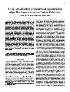
Pi ↔ P(i +t-R) mod t As an example, consider the 16-node node ring shown in Fig. 1(a) (note that the technique is applicable to any composite number of nodes, not just 16). In order to construct 2 rings of 8 nodes each (i.e., R=2, t=16, and D=8), the following links need to be added to the network (found using the two equations, Eq. (1), for each node): P 0 ↔ P 2, P 1 ↔ P 3, P 2 ↔ P 4, P 3 ↔ P 5, P 4 ↔ P 6, : : P14 ↔ P0, and P15 ↔ P1. This will result the network shown in Fig. 1(b) which consists of 2 rings of 8 nodes each. The two rings within Fig. 1(b) are formed by: (P0, P2, P4, P6, P8, P10, P12, P14) and (P1, P3, P5, P7, P9, P11, P13, P15). In addition, each node is connected to the corresponding node in the other ring (i.e., P0 ↔ P1, P2 ↔ P3, and so on). As another example, in order to construct 4 rings of 4 nodes each (i.e., R=4, t=16, and D=4), the following links need to be added to the original network shown in Fig. 1(a) (found using the equations Eq. (1) for each node): P0 ↔ P4, P1 ↔ P5, P2 ↔ P6, P3 ↔ P7, P4 ↔ P8, P5 ↔ P9, P6 ↔ P10, P7 ↔ P11, P8 ↔ P12, and so on. This will result the network shown in Fig. 1(c) which consists of 4 rings of 4 nodes each. The four rings within Fig. 1(c) are formed by: (P0, P4, P8, P12), (P1, P5, P9, P13), (P2, P6, P10, P14), and (P3, P7, P11, P15). In addition, each node is connected to the corresponding nodes in the other rings (i.e., P0 ↔ P1, P1 ↔ P2, P2 ↔ P3, P4 ↔ P5, P5 ↔ P6, P6 ↔ P7, P8 ↔
P9, and so on). All other ring configurations can be constructed in a similar way. It is important to note that the R X D mesh nearest-neighbor interconnection network is contained within each configuration. For example, the network shown in Fig. 1(b) contains within it the 2X8 (or 8X2) mesh network; similarly, the network shown in Fig. 1(c) contains within it the 4X4 mesh network. 4.2 Utilizing The MultiRing Network - Broadcasting Mechanisms. In almost all parallel problems, some form of data broadcasting is required. The MultiRing network supports broadcasting at the interconnection level. Each of the broadcasting operations performs on the order Mn on the MultiRing network, where M is the length of the message and 2n is the number of nodes. This is considered to be very efficient. This broadcast time can be shown optimal among networks which are 4-regular, to within a multiplicative constant that is independent of the size of the network. Below, three broadcasting mechanisms supported by the MultiRing are described. In the following descriptions, the node adjacent to the current node in the counterclockwise direction within a ring is referred to as the next node. i) Simple Broadcasting: In simple broadcasting, a block of data in one node is to be broadcast to all the other nodes. The operation is performed as follows (assume that A is the data to be broadcast and initially there is one ring of nodes; refer to Fig. 1(a)): one node sends a copy of A counterclockwise to the next node; reconfigure the system to yield two rings (refer to Fig. 1(b)); within each of the two rings, two nodes each send a copy of A counterclockwise to the next node; reconfigure the system to yield four rings (refer to Fig. 1(c)); within each of the four rings, four nodes each send a copy of A to the next node; continue this process n times. After n steps each of the 2 nodes will have a copy of A. ii) Tile Broadcasting: This broadcasting operation has many applications; it is a particularly useful operation for parallel pattern recognition (this broadcasting method together with the one described below have many applications in pattern recognition operations: both in low-level and high-level operations required in recognition problems). In pattern recognition problems, it is often necessary to subdivide the data into portions of data, called tiles, by horizontal and/or vertical cuts and assign each tile to a separate processor for parallel execution. If one node has a copy of all the tiles/data in its local memory, the problem is to assign particular tiles/data to particular nodes. After performing this assignment, node P0 will contain tile 0, P1 will contain tile 1, and so on. This operation is performed as follows (assuming that initially the tiles are in one node in the order: tile 0, tile 1, tile 2, and so on): send all those tiles that are numbered with an odd number n
(subscript) to the next node in the ring (only the node with all the data will perform this first task); reconfigure the system to yield two rings, within each of the two rings send all those tiles whose number (subscript) div 2 (div denotes the integer division operator) is an odd number to the next node in the ring; reconfigure the system to yield four rings, within each of the four rings send all those tiles whose number (subscript) div 4 is an odd number to the next node in the ring; continue this process n times. After n steps, node P0 will contain tile 0, P1 will contain tile 1 and so on. iii) Gossip Broadcasting: In this type of broadcasting, each node has a block of data that needs to be broadcast to all other nodes in the system. Therefore, at the end of this operation, the data in each node will be the same as the data in the other nodes; i.e., every node will have a copy of all the blocks of data. This operation is very similar to the simple broadcasting operation and is performed as follows (assuming that initially there is one ring of nodes): each node sends a copy of its data to the next node; reconfigure the system to yield two rings, within each of the two rings each node sends a copy of its data to the next node; reconfigure the system to yield four rings, within each of the four rings each node sends a copy of its data to the next node; continue this process n times.
extension of the gossip broadcast operation described earlier. vi) The master processor performs further merging at end points of polygon slices. This results in final polygon approximation. Steps iii) and v) involve communication. Each of these communications involves only n steps on
2 processor MultiRing network. a The communication overhead introduced to parallelize this application is considered to be minimal and is estimated to be about 5% of the overall execution time (excluding the initial polygon input to the MultiRing which heavily depends on the choice of input devices being used.) n
5. Mapping the polygon approximation algorithm to the multi-ring topology The reconfigurable MultiRing processor network can be effectively used to support the polygon approximation application described earlier. The MultiRing version of the algorithm presented here has been devised with scalability in mind. The mapping of the parallel polygon approximation algorithm on the MultiRing topology is described below: i) The polygon is fed into the MultiRing. One processor (loosely named the "master" processor) now contains the polygon data to be approximated. ii) The master processor divides the polygon into N polygon slices. iii) The master processor then broadcasts the polygon slices to respective multi-ring processors. This is achieved by performing the tile broadcast operation described earlier. iv) Each multi-ring processor first performs initial polygon approximation of its polygon slice. The multiring processors then perform merge operation on their resultant polygon slices. v) Each multi-ring processor, sends its results to the master processor. This is achieved by a simple
Figure 1 1.. MultiRing Topology: Topology: a 1616-node example wih three configurations
6. Results and Discussionm The original curve for polygonal approximation was traversed in a clockwise direction and extreme left point was taken as the starting point. The results of the polygon approximation can be seen in Fig 2. Without any communication, synchronization, and reconfiguration overheads, the execution of the parallel version of the algorithm presented in this paper would be p times faster (theoretical optimum) than its serial version; where p is the number of processors in the multiprocessor system. In practice, the main overhead introduced in the parallel version of this application is the communication overhead (we are assuming that the overheads associated with synchronization and reconfiguration are negligible – It has been shown that this is a reasonable assumption for
most such applications; for VLSI implementation of the reconfigurable switch, refer to [5].)
Figure 2. (a) Original curve. (b), (c) and (d) show sequential scan polygon approximation at an allowed error of 1,2,3 units respectively. (e), (f), and (g) show corresponding results using Split-and-Merge algorithm. (h), (i), and (j) show results of using Iterative algorithm. (k) and (l) show the results of the parallel algorithm.
Steps iii) and v) of mapping the parallel algorithm on the multi-ring topology involve communication (refer to Section IV – subsection C.) The communication time at step iii) is equal to the time it takes for one processor to send its whole data to only one other processor where there is a direct connection. The reason for this is that in order to perform the tile broadcast operation, first the master processor would send ½ of the data to its adjacent processor (where there is a direct link); the system is then reconfigured to yield two rings of nodes; within each inner ring, only ¼ of the slices are sent to the adjacent nodes; similarly, at each subsequent communication phase, the size of data to be transferred is halved (ie, s/2 + s/4 + s/8 + s/16 + … = s; where s is the size of the data that is being broadcast using tile broadcast operation.) The communication overhead for steps v) (refer to Section IV – subsection C) are all comparable to the overhead associated with step iii). Clearly, the overall communication overhead associated in parallelizing this application is quite minimal when compared with the processing needed. It is estimated that the overall execution of this application includes only about 5% communication overhead on typical polygon data. It should be noted that we have not considered the time it takes to initially load the input polygon data to the master processor since such time depends on the input technology being used.
Because of low communication overhead, this parallel version of the application is quite scalable (both, algorithmically and in terms of the number of processors/nodes.)
7. Conclusion The work presented here described a parallel polygon approximation algorithm targeted at reconfigurable multi-ring hardware. The algorithm is based on merging principle and grows edges simultaneously at locations where minimum merging error (local error) is produced. Merging is carried out in such a way so that both the local and the global errors are maintained within the allowed error. The parallel version of the polygon approximation algorithm targeted at reconfigurable multi-ring hardware was described. The communication overhead introduced to parallelize this application is considered to be minimal and is estimated to be about 5% of the overall execution time. Because of low communication overhead, this parallel version of the application is quite scalable (both, algorithmically and in terms of the number of processors/nodes.)
8. References [1]. Arabnia H. R., "Distributed Stereocorrelation Algorithm", international Journal of Computer Communications (Elsevier Science), pp. 707-712, 1996. [2]. Arabnia H. R., The Transputer Family of Products and Their Applications in Building A High Performance Computer, Encyclopedia of Computer Science and Technology (A. Kent and J. Williams, eds.), Marcel Dekker, New York, to appear, 1998. [3]. Arabnia, Hamid R., and Thiab R. Taha A Parallel Numerical Algorithm on a Reconfigurable Multi-Ring Network. Journal of Telecommunication Systems, Vol. 10, pp. 185-203, 1998. [4]. Bhandarkar S. M. and Arabnia H. R., "Parallel Computer Vision on a Reconfigurable Multiprocessor Network"; The IEEE Transactions on Parallel and Distributed Systems, Vol. 8, No. 3, pp. 292-310, 1997. [5]. Bhandarkar S. M., Arabnia H. R. and Smith J. W., “A Reconfigurable Architecture for Image Processing and Computer Vision”, Special Issue of International Journal of Pattern Recognition and Artificial Intelligence (IJPRAI) on “VLSI Algorithms and Architectures for Computer Vision, Image Processing, Pattern Recognition and AI”, Vol. 9, No. 2, pp. 201229, 1995. [6]. Dunham, J. G., "Optimum uniform piecewise linear approximation of planar curves," IEEE Trans. Pattern Anal. Machine Intell., vol. PAMI-8, pp. 67-75, 1986.
[7]. Lowe, D. G., "Organisation of Smooth Image Curves at Multiple Scales," In Proc. 2nd ICCV, Tarpon Springs, FL, pp. 558-567, 1998. [8]. Pavlidis, T., "Waveform segmentation through functional approximation," IEEE Trans. Comput., vol c-22, pp. 689-697, 1973. [9]. Pavlidis, T., and Horowitz, S. L., "Segmentation of plane curves," IEEE Trans. Comput. , vol. c-23, pp. 860-870, 1974. [10]. Pavlidis, T., Algorithms for Graphics and Image Processing. Springer Verlag, 1982. [11]. Ramer, U., "An iterative procedure for the polygonal approximation of plane curves, "Comput. Graphics Image Processing, vol. 1, pp. 244-256, 1972. [12]. Roberge, J., "A data reduction algorithm for planar curves," Comput. Vision, Graphics, Image Processing, vol. 29, pp. 168-195, 1985. [13]. Sklansky, J. and Gonzalez, V., "Fast polygonal approximation of digitised curves," Pattern Recognition, vol. 12, pp. 327-331, 1980. [14]. Sun Yung-Nien and Huang Shu-Chien, “Genetic Algorithms for Error-Bounded Polygon Approximation, International Journal of Pattern Recognition and Artificial Intelligence, Vol. 14, No. 3, pp. 297-314, 2000. [15]. Suzuki, K., Nishida, Y., and Hata, S., "A fast polygonal approximation method for real-time shape recognition," IEEE Conference on Pattern Recognition, pp. 388-394, 1986. [16]. Teh, C. and Chin, R. T., "On the detection of dominant points on digital curves," IEEE Trans. Pattern Anal. Machine Intell., vol. 11, issue 8, pp. 859872, 1989. [17]. Wall, K. and Danielsson, P. E., "A fast sequential method for polygonal approximation of digitized curves," Comput. Vision, Graphics, and Image Processing, vol. 28, pp. 220-227, 1984. [18]. Wani M. Arif and Pham D.T., "Feature-based control chart pattern recognition", Int. J. Prod. Res., 35(7), pp1875-1890, 1997. [19]. Wani M. Arif and Pham D. T., “Efficient Control Chart Pattern Recognition Through Synergistic and Distributed Neural Networks”, Proceedings of Mechanical Engineers, Journal of Engineering Manufacture, pp 157-169, vol. 213, part B, 1999. [20]. Wani, M. Arif, “SAFARI : A Structured approach for automatic rule induction” IEEE Transactions on Systems Man and Cybernetics journal. Vol 31 (4): pp 650-657 AUG 2001. [21]. Wani, M. Arif, and Batchelor B. G., “Edge Region Based Segmentation of Range Images”, IEEE Transactions on Pattern Analysis and Machine Intelligence, pp. 314-319, March 1994. [22]. Wani, M. Arif, and Arabnia, H. R., “Parallel Edge-Region-Based Segmentation Algorithm Targeted at Reconfigurable Multi-Ring Network,”, The Journal
of Supercomputing, vol. 25, iss 1, pp. 43-63 , May 2003. [23]. Williams, C. M., "An efficient algorithm for the piecewise linear approximation of planar curves," Comput. Graphics Image Procesing, vol. 8, pp. 286293, 1978. [24]. Wu, L. D., "A piecewise linear approximation based on a statistical model," IEEE Trans. Pattern Anal. Machine Intell., vol. PAMI-6, pp. 41-45, 1984.