1070
IEEE SIGNAL PROCESSING LETTERS, VOL. 22, NO. 8, AUGUST 2015
Locality-Constrained Sparse Auto-Encoder for Image Classification Wei Luo, Jian Yang, Wei Xu, and Tao Fu
Abstract—We propose a locality-constrained sparse auto-encoder (LSAE) for image classification in this letter. Previous work has shown that the locality is more essential than sparsity for classification task. We here introduce the concept of locality into the auto-encoder, which enables the auto-encoder to encode similar inputs using similar features. The proposed LSAE can be trained by the existing backprop algorithm; no complicated optimization is involved. Experiments on the CIFAR-10, STL-10 and Caltech-101 datasets validate the effectiveness of LSAE for classification task. Index Terms—Feature learning, image classification, sparse auto-encoder.
I. INTRODUCTION
E
NCODING local features based on an overcomplete dictionary with sparse constraints on their codes has gained much attention in the field of vision study. This implementation mainly involves two issues: learning a dictionary ( ) and encoding a local feature ( ) based on to obtain its sparse code ( ). This problem can be formalized as (sparse model) and solved by alternatively iterative opis fixed, timization scheme. After training is accomplished, then new comings only need to be optimized based on to obtain their sparse codes. The sparse model faces problems for large scale and real-time applications, in spite of its big successes in various vision applications, e.g. image denoising, super-resolution, classification, because it does not contain an encoder module but only includes a decoder module. The encoder module is replaced by an optimization procedure to obtain codes in the sparse model. To speed up the process of computing sparse codes, Ranzato et al. [1] introduced a Sparse Auto-Encoders (SAE), which explicitly includes a linear encoder module and a nonlinear transformation module. The encoder outputs a group of responses by multiplying inputs and the weight matrix, and the transformation module employs logistic sigmoid units to transform these responses into quasi-binary sparse codes. So after the learning is accomplished, a simple feed-forward operation can get the sparse code. Coates et al. [2] proposed a more intuitive SAE, which directly constrains the average response of each hidden unit of the encoder to a small value. The learning in [2] can be Manuscript received October 31, 2014; revised December 10, 2014; accepted December 16, 2014. Date of publication December 18, 2014; date of current version January 08, 2015. The associate editor coordinating the review of this manuscript and approving it for publication was Prof. Tolga Tasdizen. The authors are with the School of Computer Science and Engineering, Nanjing University of Science & Technology, Nanjing 210094, China (e-mail:
[email protected];
[email protected];
[email protected]) Color versions of one or more of the figures in this paper are available online at http://ieeexplore.ieee.org. Digital Object Identifier 10.1109/LSP.2014.2384196
easily conducted by using the backprop algorithm [3], while alternatively optimization is employed in [1], because the weights and the transformed codes are coupled. The aforementioned sparse model and SAE are all based on reconstruction error, which is suitable for low-level vision applications. However, it is more advisable to exploit the relationship between coding and recognition for higher-level recognition tasks, e.g. classification. This viewpoint has been proved in the field of image classification, where locality is more essential than sparsity, as locality must lead to sparsity but not necessary vice versa [4]. To this end, Wang et al. [4] proposed the Locality-constrained Linear Coding (LLC) that first searches the -nearest bases of an input in the dictionary and then reconstructs it using these bases by solving a constrained least square fitting problem. The same coding strategy was also advocated by Salient Coding (SaC) [5] and Localized Soft-assignment Coding (LSC) [6], but both of them do not contain a dictionary learning module and thus they rely on a dictionary trained by other procedures, e.g. K-means. While LLC includes a dictionary learning module, the learning efficiency is constrained by the size of the dictionary and a predefined threshold value. With a large dictionary and a small threshold value, LLC costs much for dictionary learning. We propose a simple yet efficient SAE in this study, which has the property of retaining the similarity of codes for similar inputs and forming the features (weight matrix) as a local subspace of training data. The proposed SAE only retains code units of the encoder, whose corresponding features are the -nearest neighbors of the input, and sets the others to zero. Then the decoder takes the code units to reconstruct the input. Based on this operation, the learning practically forces the features to form a local subspace of training data. To determine the -nearest neighbors of an input, the proposed SAE normalizes each inner production between a feature and the input by dividing the norm of the feature. And then the -nearest neighbors are determined by the top- normalized values. Experiments on image classification validate the effectiveness of this coding strategy adopted by the proposed SAE. For simplicity, the proposed SAE is called Locality-constrained SAE (LSAE). Exploiting the structure of the auto-encoder (AE) for learning can alleviate the phenomenon of dead features in locality based learning models, in which earlier updated features have the advantage of being the neighbors of inputs than random features. This phenomenon causes the learning mainly focus on the earlier updated features and leaves the others with low probability to be updated. This problem was noticed in LLC, and the author utilized the whole dictionary for coding to update the dictionary. For this reason, the dictionary learning is expensive in LLC. Here we take advantage of the AE structure to explicitly force each hidden unit to possess sparse responses to implicitly update each feature according to equal probability, and thus
1070-9908 © 2014 IEEE. Personal use is permitted, but republication/redistribution requires IEEE permission. See http://www.ieee.org/publications_standards/publications/rights/index.html for more information.
LUO et al.: LOCALITY-CONSTRAINED SPARSE AUTO-ENCODER
1071
circumventing the phenomenon of dead features. We incorporate this constraint in the backprop to train our LSAE in this study. Comparing to the LLC dictionary learning, the learning in LSAE is simple and effective. II. THE MODEL In this section we present LSAE and uncover the properties of the model by discussing different activation units, regularization methods and parameters. A. Locality-Constrained Sparse Auto-Encoder (LSAE) as the input, and as the Let us denote code, where is in general greater than (for overcomplete representations). Let the weights in encoder and decoder be the columns of matrix , which means tied weights are used. And let and be the biases in the encoder and decoder, respectively. Then, the encoder and decoder respectively compute and in AE as: (1) where is a component-wise nonlinear function and is the reconstructed input. In order to introduce locality into the process of coding, LSAE works as: (2) and . We choose where as the rectified linear unit (ReLU): , in this study except for a explicit specification, and discuss the effects of other activation units in Section II-B. is a set operator and it only retains components of , whose corresponding features are the nearest neighbors of the input , and sets the other components to zero. (3) can be deterSpecifically, the -nearest neighbors of in . The influmined by the top- projections: ence of different on the properties of LSAE is discussed in Section II-D. Then during training we minimize:
(4) where is the number of training samples and is a sparsityinduced regularization term, which is discussed in Section II-C. is a penalty parameter for regularization. LSAE can be trained using the backprop algorithm [3], which updates weights and bias by back propagating the reconstruction error gradient from the output layer to the input layer. Comparing to SAE [2], the only change in gradient computation is the gradient for features that is caused by the projection operation. In LSAE, for a hidden unit , its gradient for correis: sponding feature (5)
where . As we use ReLU in LSAE, is set to 0 when and 1 when as in [7]. When training is accomplished, sparse codes can be easily get by a simple feed-forward operation. (We provide a detail back propagation process of LSAE in the supplementary materials.) Properties: Normalizing features in the encoder when computing the code is essentially replacing the inner production, , in AE by projection, . This operation explicitly makes the search for neighbors of an input become feasible. Because the length of features are not normalized in AE and SAE, the inner production cannot be used to determine neighbors of an input. On the contrary, normalizing features in each iteration makes less clear which objective function is minimized in learning as explained in [1]. The normalization also implicitly makes the bias term of hidden units capture the distances between predicted codes and idea codes (system uncertainty) more precisely, because the projection is not affected by the length of features. With small in LSAE, e.g. , each feature will only have a small number of samples to be its neighbors in the batch learning model, so the bias term can capture very precise system uncertainty, which causes the learning in LSAE is very fast (see Section III). For this reason, we can employ ReLU as the activation unit in LSAE for codes prediction. This property of LSAE will disappear with a large , and a more strong nonlinear-degree unit is needed to predict codes in this case. We study this problem in the next Section. B. Secrets Behind Different Activation Units The properties of different activation units have been fully studied in [3]. And recent studies in deep networks [7], [8] advocate ReLU for its ability to preserve much more information. We here argue that only those activation units with strong ability to handle the system uncertainty, which is failed to be captured by the bias, can successfully learn features in reconstruction-based SAE. Because the length of features are not normalized in SAE, the bias cannot precisely capture the system uncertainty. Thus, SAE needs a strong nonlinear function to complement the uncertainty for feature learning. We experiment on whitened natural images with different sigmoids and ReLU, and tune the learning rate and sparsity penalty range from 0.001 to 0.1 and 0.0001 to 5, respectively. We only observe the logistic sigmoid unit has the ability to learn features in SAE, due to its strong degree of nonlinearity (see Fig. 2). The logistic sigmoid unit can be used to learn better features if the bias term can capture the system uncertainty more precisely in SAE. To this end, we experiment on a LSAE with logistic sigmoids and without locality constraint. The learned features are shown in the first figure of Fig. 1. Comparing to features learned in SAE, we conclude the projection leads the bias term to capture more precise system uncertainty. We then further experiments on LSAE but with varying . Since the nonlinear-degree of ReLU is weaker than that of logistic sigmoid, LSAE fails to learn useful features when is large. But with decreasing, the bias in LSAE can capture the system uncertainty more precisely, thus the learned features become better and better. We demonstrate our results on natural images in Fig. 1, but the same effects are also observed on other datasets, such as on CIFAR-10, MNIST. C. Understanding the Regularization Term In LSAE, the sparse responses of hidden units are obtained by the locality constraint instead of by the sparsity-induced reg-
1072
Fig. 1. Randomly selected 36 out of 256 features learned on natural images. The left two figures are features learned by LSAE with logistic sigmoids and ). The right two figures ReLU, respectively (without locality constraint, and 5, respectively. are features learned by LSAE with ReLU and
IEEE SIGNAL PROCESSING LETTERS, VOL. 22, NO. 8, AUGUST 2015
Fig. 3. Left: Randomly selected 36 out of 256 features learned on the MNIST , right: . Learning parameters: dataset with different . left: . Right: Recognition rate with varying .
III. EXPERIMENTS A. Datasets and Experimental Setup
Fig. 2. Randomly selected 36 out of 256 features learned on natural images. The first two figures are features learned by SAE with KL-divergence and regularizer, and the last two figures are features learned by LSAE with reguand 0.1, respectively. The average length of features for each larizer and method is: 3.38,3.43,0.73 and 0.92.
ularization. We argue that the sparsity-induced term is essentially forcing each feature to have an approximately equivalent probability to be updated. We employ the norm, , as regularization in our implementation, because ReLU can produce exact 0 response and it’s a non-saturated function. While the logistic sigmoid can cooperate with KL-divergence to constrain sparse responses of hidden units and force each feature to be updated in SAE [2], it does not generate exact 0 responses and causes the norm of features are bigger than 1 to compensate the information suppression problem in saturated units [8] (see Fig. 2). The norm encourages each hidden unit to have the lifetime sparsity as that in sparse filtering [9], which implicitly forces each feature to be updated. To verify this, we first experiment on natural images by using SAE with KL-divergence and regularizer, respectively. We find the regularizer works as well as KL-divergence does in SAE to force each feature to be updated. We then compare the features learned by LSAE with and without regularizer. We find LSAE with regularizer learns better features and the length of features are approximate to 1 (see Fig. 2). D. The Influence of The hyper-parameter is used to determine how many local features of an input are used to reconstruct it. Because of the locality, the local features form a local subspace of training data during training. Therefore, we can expect the learned features are similar to training samples when is small. And with increasing, it becomes difficult to learn a local subspace, thus the learned features degenerate to basic elements of training data. We, therefore, argue that the proposed SAE has the ability to find a local subspace of training data. Empirical experiments on MNIST [10] validate our conjecture. As shown in Fig. 3, the features are similar to the training samples with small , while they resemble digit strokes with large . Further, to justify the importance of locality in coding, we evaluate the performance with varying for classification tasks. As analysed in the properties of LSAE, the recognition rate decreases with increasing (see Fig. 3).
color images in 10 CIFAR-10 [11] consists of 60,000 classes. There are 50,000 training images and 10,000 test images. STL-10 [2] comprises 10 classes of color images, and has a total of 5,000 training samples, but only 1,000 samples are permitted to use in each trial for a total of 10 trials. There are 8,000 test images and 100,000 unlabeled examples for unsupervised learning. Training on this two datasets is as follows: 1) We randomly sample 100,000 patches (for STL-10, we downsample the images into size of ) and whiten them for training LSAE. 2) We densely extract patches with stride 1 for each image and map them into sparse codes via LSAE. 3) For each image, we use max-pooling to pool the codes in each of the 4 quadrants and concatenate them to form an image feature for training linear SVMs. For CIFAR-10 and STL-10, randomly selected 4,500 training samples from each class and 4,000 samples from the training set are used to train classifiers using features generated by different LSAEs ( and ), and the rest 5,000 and 1,000 samples are used to determine the best LSAE, respectively. The Caltech-101 contains 9,144 images belonging to 101 object categories and one background category. We randomly compute 100,000 SIFT features and normalize each dimension by subtracting the mean value for learning LSAE. After this, we evaluate the performance of image features generated by different LSAEs using 30 images from each class with 5-folder cross validation. Image features are generated by 1) extracting SIFT features with a step size of 8 pixels, 2) subtracting the mean value and map them to codes via LSAE, 3) max pooling the codes in each of the , , subregions and concatenating them. After obtaining the best LSAE on training samples, we retrain the linear SVMs using all training samples and test on no more than 50 images from each class and report the average classification accuracy on 5 random trials. B. Learning Efficiency Evaluation We evaluate the learning efficiency of LSAE with comparison to SAE and LLC on natural images [12] (256 features). Training data are 100,000 whitened patches. Table I summarizes the learning parameters and total training time for each method. We stop the learning algorithm once the average reconstruction error between two consecutive iterations is smaller than 0.05. Specifically, LSAE converges the most fast with 9 epochs and 11.2 seconds per epoch, while LLC and SAE+KL ( ) take 5 and 20 (21) epochs with 149 and 6.2 (5.4) seconds per epoch, respectively. Further, dead features are difficult to avoid in LLC, while this can be easily circumvented in LSAE through introducing constraint on hidden units. (see supplementary materials)
LUO et al.: LOCALITY-CONSTRAINED SPARSE AUTO-ENCODER
1073
TABLE I PERFORMACE ON LEARNING EFFICIENCY
TABLE IV PERFORMACE ON CALTECH-101
is initial velocity, represents the threshold value used in LLC. Experimental environment: 4 3:2 GHz i5 cores and 8G RAM, Matlab. Parameters for LSAE:
;
;
;
.
TABLE II PERFORMACE ON CIFAR-10
Parameters for LSAE:
;
;
;
.
TABLE III PERFORMACE ON STL-10
Parameters for LSAE:
;
;
;
.
to capture prior knowledge of training data by comparing it with locality-constrained optimization based sparse coding methods. We report the results of LLC [4], SaC [5], LSC [6] by reimplementing the public available codes. The others come from their original work. All methods are trained with 1024 features. The results are demonstrated in Table IV. In comparison, LSAE achieves accuracy, which is competitive with that of LSC and outperforms the results of all other dictionary learning and locality based methods. IV. CONCLUSION In this work, we studied a new encoding method for learning SAE and proposed a corresponding locality-constrained SAE. We explored the properties of LSAE and empirically validated its ability for feature learning. Comparing to previous SAE, LSAE can also be trained by the backprop algorithm and has the ability to find a local subspace of training data, which enables it to encode similar inputs using similar features. Experiments on classification tasks further validated its effectiveness. REFERENCES
C. Performance on CIFAR-10 The classification performance in Table II verifies the effectiveness of LSAE. Comparing to SRBMs, SAE seems to systematically perform better. However, LSAE outperforms SAE. Although LSAE and SAE share many commons, the locality constrained coding in LSAE obviously brings advantages. Even comparing to the more complicated alternative optimization based SAE [1], LSAE can achieve the same performance with a much lower dimensional code (3200 vs. 1600). From Table II, LSAE obtains 72.7% and 74.7% accuracy with 1024 and 1600 features, respectively. This performance is further elevated to with 3200 features. D. Performance on STL-10 As previous relevant work (to SAE) rarely reports results on this dataset, we compare the classification performance with some other feature learning methods which had reported their results. The results are shown in Table III. The K-means (Triangle) obtains accuracy with 1600 features in [2], whereas LSAE achieves with only 1024 features, and the performance is improved to and with 1600 and 3200 features, respectively. This result also surpasses the results obtained by Reconstruction ICA (RICA) [13] and Sparse Filtering (SF) [9], which are experimented on the full resolution images. E. Performance on Caltech-101 For the limited training samples, SAE was seldom tested on this dataset. We here validate LSAE has a strong learning ability
[1] M. Ranzato, Y.-L. Boureau, and Y. LeCun, “Sparse feature learning for deep belief networks,” NIPS, 2007. [2] A. Coates, H. Lee, and A. Y. Ng, “An analysis of single-layer networks in unsupervised feature learning,” in Int. Conf. Artificial Intelligence and Statistics, 2011. [3] Y. LeCun, L. Bottou, G. B. Orr, and K.-R. Müller, , G. Montavon, G. B. Orr, and K.-R. Müller, Eds., “Efficient backprop,” in Neural Networks: Tricks of the Trade, 2nd ed. Berlin, Germany: Springer, 2012, pp. 9–48. [4] J. Wang, J. Yang, K. Yu, F. Lv, T. Huang, and Y. Gong, “Localityconstrained linear coding for image classification,” CVPR, 2010. [5] Y. Huang, K. Huang, Y. Yu, and T. Tan, “Salient coding for image classification,” CVPR, 2011. [6] L. Liu, L. Wang, and X. Liu, “In defense of soft-assignment coding,” ICCV, 2011. [7] V. Nair and G. E. Hinton, “Rectified linear units improve restricted boltzmann machines,” ICML, 2010. [8] X. Glorot, A. Bordes, and Y. Bengio, “Deep sparse rectifier neural networks,” in Int. Conf. Artificial Intelligence and Statistics, 2011. [9] J. Ngiam, P. W. Koh, Z. Chen, S. Bhaskar, and A. Y. Ng, “Sparse filtering,” NIPS, 2011. [10] Y. LeCun, L. Bottou, Y. Bengio, and P. Haffner, “Gradient based learning applied to document recognition,” in Proc. IEEE, 1998, vol. 86, no. 11, pp. 2278–2324. [11] A. Krizhevsky, Learning multiple layers of features from tiny images Univ. Toronto, Toronto, ON, Canada, Tech. Rep., 2009. [12] P. Arbelaez, M. Maire, C. Fowlkes, and J. Malik, “Contour detection and hierarchical image segmentation,” IEEE Trans. Patt. Anal. Mach. Intell., 2011. [13] Q. V. Le, A. Karpenko, J. Ngiam, and A. Y. Ng, “Ica with reconstruction cost for efficient overcomplete feature learning,” NIPS, 2011. [14] A. Coates, A. Y. Ng, and A. Y. Ng, “The importance of encoding versus training with sparse coding and vector quantization,” in ICML, 2011.