Localization of Wireless Sensor Network Using Artificial Neural Network Mohammad Shaifur Rahman, Youngil Park, and Ki-Doo Kim* Dept. of Electronics Engineering Kookmin University, Seoul, 136-702, Korea Tel: +82-02-910-5073, Fax: +82-02-910-4645 * E-mail:
[email protected]
Abstract— In Wireless Sensor Networks (WSN), location estimation is important for routing efficiency and location-aware services. Traditional received signal strength based localizations using propagation-loss model are often erroneous for the lowcost WSN devices. The reason is that the wireless channel is vulnerable to so many factors that deriving the appropriate propagation-loss model for the low cost WSN devices is not possible. Hence, we propose a flexible model based on neural network and grid sensor training phase for accurate localization of sensors. Simulation results show that the location accuracy can be increased by increasing the grid sensor density and the number of access points.
I.
localizations are being pursued as a cost-effective alternative to more expensive range-free approaches. TOA-based technique employs the signal transmission time from the Access Points (AP) to the sensor nodes to get the distance estimation. However, precise time synchronization is needed in the network which is achieved by installing Global Positioning System (GPS) or atomic clock on APs. In AOAbased technique, the sensor nodes should have the capability of sensing the direction from which the signal is received. It requires several ultrasound receivers or an antenna array which may be expensive as well as may cause blind spots. TDOA measures the delay time of the signal arrival. Hence, AP clock should have to be faster and synchronized enough to respond to this fractional quantity of time. Both TOA and TDOA require synchronization setting which is infeasible for the inexpensive sensor nodes to provide fine-grain time synchronization. Since the indoor environment is complex with noise, multipath affect and Non Line of Site (NLOS) properties, AOA, TOA and TDOA techniques cannot get the desirable accuracy in indoor sensor network deployment. RSSI, on the other hand, estimates the distance by the RFpropagation loss model which does not need any additional sensor/actuator hardware and it has been studied for several years as a low-cost localization technique. Hence, we work on the RSSI-based location estimation technique which is most appropriate for inexpensive sensor nodes. In this technique, a simple mathematical expression represents the relationship of the distance among the sensor nodes. However, wireless channel is influenced by so many parameters that deriving the appropriate propagation-loss model for off-the-shelf low cost WSN devices is not possible. Hence, we are motivated to consider flexible models based on networks of functions such as Neural Network (NN). The non-linear transfer function and sufficiently large number of neurons guarantee the capability of the network for representing the relationship among the inputs (signal strengths) and outputs (position). We propose a new algorithm for location estimation of WSNs using Multi-Layer Perceptron (MLP) NN. In the proposed algorithm, the network is trained by using stationary reference sensors installed in grid arrangement (hereafter termed as grid sensors), the location of which is known. RSS values at all the APs from the grid sensors and the known location of the grid sensors are used to train the network. The
INTRODUCTION
In recent years, research on wireless sensor network (WSN) has gained an increasing interest. Advancements in radio communication and micro-electronics have enabled the development of micro-sensors that can manage wireless communication. WSN can be deployed in a large area for monitoring environmental parameters, such as pressure, temperature, humidity, luminosity, air quality, soil property, etc. Most of the environmental sensing applications need to have location information of sensor nodes because sensing data are meaningless without it. Many communication protocols of the WSNs are also based on the location information of the sensor nodes. Location-aware applications such as navigation, autonomous robot movement, and asset tracking require localization. Hence, location estimation is a significant technical challenge for the researchers. Several algorithms and techniques have been proposed for sensor network location estimation. All these techniques can be divided into two broad categories based on the type of information used in localization: range-based and range-free. Range-based techniques need point-to-point distance or angle information to calculate the location which is done by Triangulation or Trilateration. Received Signal Strength (RSS), Angle of Arrival (AOA), Time of Arrival (TOA), and Time Difference of Arrival (TDOA) are four important techniques to get the distance estimation. Range-free techniques do not need distance information; rather they estimate the location depending on the information of proximity of the reference nodes. Due to the hardware limitation of inexpensive WSN devices, range-based
978-1-4244-4522-6/09/$25.00 ©2009 IEEE
639
ISCIT 2009
training is updated in a regular interval of time to incorporate the changes in wireless channel to ensure the consistency of the localization. Error back propagation training is performed using the Levenberg-Marquardt algorithm. Simulation results show that the accuracy of the localization largely depends on the density of grid sensors and number of APs. Some previous works of localization based on RSS and NN are briefly described in the following section. II.
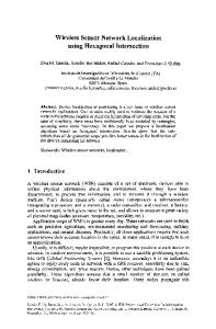
Neural networks are modeled resembling the biological neuron system. It is the network of interconnected nodes, termed ‘Neurons’, with linear or nonlinear active functions. Various types of networks can be created by varying the activation functions of the neurons and the structure of the weighted interconnections among them. MLP is a widely used NN class. Adjusting the weights requires a learning strategy that starts from a set of labeled examples to construct a model that will then be generalized in an appropriate manner when confronted with new data, not present in the training set. The architecture of the multi-layer perceptron is shown in Fig. 1. The signal flows sequentially through the different layers (input, hidden, and output) from the input to the output layer. Each layer contains one or more neurons and every neuron contains a transfer function. Each neuron calculates a scalar product between a vector of parameters (weights) and the vector given by the outputs of the previous layer. The result is then applied to the transfer function to produce the input for the next layer. Normally, the hidden layers contain sigmoid transfer function while the output layer contains linear function, so that output is not bound. It has been shown that a network of a single hidden layer having adequately large number of neurons is sufficient to approximate any continuous function with the desired accuracy [6]. In our study, we have investigated several network configurations and activation functions. After a series of tests, it is seen that MLP network with 2 hidden layers (10 neurons in the first hidden layer and 4 neurons in the second hidden layer) and tan-sigmoid transfer function gives better estimation in the present study.
RELATED WORKS
RADAR location system was proposed by Microsoft Research which used the IEEE 802.11b WLAN technology [1, 2]. In this system, RSS is used for determining distance between AP and mobile terminal. The position is then calculated by triangulation with both an empirical method and a signal propagation modeling method. Results show that the empirical method is superior in terms of accuracy with median resolution within the range of about 3 meters. On the other hand, the signal propagation modeling method shows 4.3 meters median accuracy. SpotON, another RSS-based location sensing system uses RFID active tags and AIRID base stations [3]. This system is similar to RADAR system proposed by Microsoft and it develops a fine grained tagging technology based on RF signal strength. J. Astrain et al. modeled uncertainty in RSS measurements as fuzzy sets by dividing the area of interest into zones [4]. A radio map is developed offline and is used to train the fuzzy inference system. There are six fuzzy sets for RSS: Excellent, Very Good, Good, Low, Very Low, and None. The degree of membership of a mobile device of a specific area is used to determine the location estimate which provides the accuracy of about 90%. A generalized regression neural network with one hidden layer is used for a pattern matching algorithm by C. Nerguizian et al. [5]. Measured RSS value for each access point and corresponding location are used to train the network. The maximum error among estimated and true positions for the test data was 43.2 meters. The location accuracy, applied in an in-building environment, has been found to be 0.5 meter for 90% of trained data and about 5 meters for 45% of untrained data. Motivated from [5], we propose the grid sensor algorithm for Levenberg-Marquardt error back propagation training of NN for localization of WSNs. In this work, both Line of Sight (LOS) and Non Line of Sight (NLOS) condition in indoor environment has been considered. Here, we do not need any special purpose equipment besides the WSN devices, while the flexible modeling and learning capabilities of neural network achieve lower errors in determining the position. Also, learning can be updated with the change in wireless channel condition. III. A.
B.
Network Training To approximate a function, the MLP network is trained by repeatedly passing forward the input through the network. The weights are updated based on the difference between the desired output and the actual output of the network. Final weights of the MLP network completely depend on the initial weights. Finding the sets of weights to get the best performance is a great challenge and it ultimately turns into
NEURAL NETWORKS
Fig. 1. Multi-layer perceptron neural network architecture. Inputs are the received signal strength values from a particular sensor and measured by different access points. Output is the location
Network Architecture
640
trial and error procedure. It is essential to note that the objective of the training algorithm is to build a model with good generalization capabilities when confronted with new input values, values not present in the training set. Among all simulated data sets, 60% are randomly extracted for training purpose, 20% for validation purpose and the remaining 20% for test purpose. There are many variations of error back propagation algorithms for training the network. In our present study, we apply Levenberg-Marquardt training algorithm.
d 0 to be 1 m. The path-loss for reference distance is taken as 30dB. Path-loss distance exponent γ is assumed 2.1, and the transmit power is 10dB. The random variation of RSS is expressed as a Gaussian random variable of zero mean and variance of σ 2 . In order to generate shadowing effects, the value for the standard deviation, σ is selected to be 7 for LOS condition and 9.7 for NLOS condition. All the assumptions used in this work are taken from [8]. Two training matrices are formed from the simulation namely input and target matrices. The input matrix contains the RSS column vectors for every grid sensor. Each RSS vector is composed of RSS values obtained from all the APs. The target matrix contains the known locations of the grid sensors. We used MATLAB for the simulation. The performance criterion of the algorithm is the Root Mean Square Error (RMSE) given by:
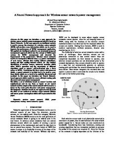
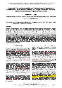
IV. WSN SIMULATION ENVIRONMENT To train the network, a WSN containing 8 APs and 81 grid sensors are arranged in an square area of 200m × 200m as shown in Fig. 2. The APs are set at the edges of the squared area and 81 sensor nodes are set in grid arrangement. All the sensor nodes are in the reading range of all the access points, i.e. all the nodes are within one hop distance of all the APs. The network operating frequency is 2.4 GHz ISM band. In order to generate the RSS samples as a function of distance for the network training, a path loss model with log-normal shadowing effects is used [7]: d L = L0 + 10γ log10 + X g , where L is the total path-loss d0
e12 + e2 2 + L + en 2 , where n is the number of n −1 trials estimating the location of the sensor node and e1 , e2 L en are the location errors as Euclidian distances between the location estimate and the actual location of the sensors. RMSE =
V.
measured in Decibels (dB), d is the length of the path in meter, d 0 is the reference distance in meter, L0 is the pathloss at the reference distance d 0 in dB , γ is the path-loss distance exponent, X g is a random variable with zero mean,
The performance of the proposed sensor grid algorithm is evaluated for localization accuracy by simulation experiments. First experiment is performed to evaluate the influence of grid sensor density on the accuracy of the localization. 8 Aps and 81 grid sensors are placed in the simulation area ranging from 20 × 20 m 2 to 200 × 200 m 2 with a step of 20 × 20 m 2 . The RSS vectors and the known location coordinates of the grid sensors are used to train the network. After the training, the
reflecting the attenuation (in dB) caused by flat fading. To consider the indoor environment, we assume the value for 240 Sensor Nodes
220
200
Access Points
200
180
180
160
Unknown Nodes
Estimated Positions
140
140 120
Distance (m)
Distance (m)
160
100 80 60
120 100 80
40
60
20
40
0 -20 -20
SIMULATION RESULTS
20 0
20
40
60
80 100 120 140 160 180 200 220
0
Distance (m)
0
20
40
60
80
100 120 140 160 180 200
Distance (m)
Fig. 2. Location of the Access Points (AP) and grid sensors indicated by the solid circles and squares, respectively. RSS from 8 APs and 81 grid sensors are used for training the network.
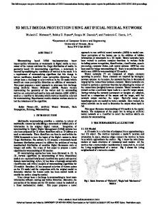
Fig. 3. Location of the actual and estimated sensors indicated by the hollow squares and triangles, respectively.
641
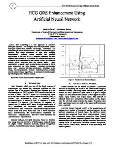
network is used to locate 41 unknown sensors placed randomly in the same area. Fig. 3 shows the actual and estimated locations of the 41 unknown sensors represented by the square- and triangle-symbols, respectively. Here, the RMSE was about 4.6 m for LOS condition. Since, number of APs and grid sensors are kept unchanged, the density of the grid sensors decreased as we increased the area. Simulation experiments show that the RMS error in terms of distance is increased with decreasing the sensor density. It is shown in Fig. 4 that the RMSE increases from 0.54 to 5.1 m in case of LOS condition and from 0.69 to 6.1 m in case of NLOS condition when the area is increased from 20 × 20 m 2
to the number of APs, which is shown in Fig. 5. RMSE is found to be decreased from 6.854 to 2.5 m for LOS condition and from 8.69 to 3.16 m for NLOS condition, when the number of APs is increased from 3 to 8. VI. CONCLUSIONS In this paper, we propose and investigate a localization technique for WSNs using NN. We consider the NN for building a flexible mapping between RSS and position of the sensor nodes. In this technique, the NN is trained using the RSS values of the grid sensors. The positive features of the system are its reliance against the change in the RSS measurements with time and no need of extra arrangement of hardware. The network training is updated with regular interval of time to minimize location error. Simulation experiments show that the location accuracy can be increased by increasing the grid sensors density and APs.
to 200 × 200 m 2 . From this experiment, it can be assumed that localization accuracy can be increased by increasing the grid sensors. In our second experiment, relationship of the number of APs with the location accuracy is investigated. The number of APs is increased from 3 to 8. As a result, RSS vector components increased from 3 to 8 as well. It is found in this simulation that the location accuracy is directly proportional
Root Mean Square Error (m)
6
ACKNOWLEDGMENT This work was supported by the National Research Foundation of Korea (NRF) grant funded by the Korea government (MEST) (No. 2009-0083890).
LOS NLOS
5
REFERENCES [1] P. Bahl and V. N. Padmanabhan, “RADAR: An in-building RFbased user location and tracking system,” In Proceedings of IEEE INFOCOM 2000, pp. 775–784, March 2000.
4 3
[2] K.Whitehouse, C.Karlof, and D.Culler, “A practical evaluation of radio signal strength for ranging-based localization”, Mobile Computing and Communications Review, vol. 11, No. 1, pp. 4152, January 2007.
2 1 0 20
40
60
80
100
120
140
160
180
[3] J. Hightower, G. Borriello, and R. Want, “SpotON: an indoor 3D location sensing technology based on RF signal strength. The University of Washington, Technical Report: UW-CSE 2000-02-02, February 2000.
200
2
Dimension of Indoor Space (n*n m )
Fig. 4. Root mean square error Vs dimension of the area. The number of access points and grid sensors are kept same. Hence, grid sensor density is decreased with increasing the area.
9
LOS NLOS
8 Root Mean Square Error (m)
[4] J. Astrain, J. Villadangos, J. Garitagoitia, J. Mendivil, and V. Cholvi, “Fuzzy location and tracking on wireless networks,” In Proceedings of the 4th ACM International Workshop on Mobility Management and Wireless Access, pp. 84-91, October 2006. [5] C. Nerguizian, C. Despins, S. Affes , “Indoor geolocation with received signal strength fingerprinting technique and neural networks,” Telecommunications and Networking - ICT 2004, vol. 3124/2004, pp. 866–875, 2004.
7 6 5
[6] K. Hornik, “Approximation capabilities of multilayer feedforward networks,” Neural Networks, vol. 4, No. 2, pp. 251–257, 1991.
4 3
[7] T. S. Rappaport, Wireless Communications: Principles and Practice, Prentice Hall, 2002.
2 3
4
5
6
7
8
Number of Access Points
[8] Y. K. Lee, E. H. Kwon, and J. S. Lim, “Self location estimation scheme using ROA in wireless sensor networks,” Embedded and Ubiquitous Computing, Springer, vol. 3823/2005, pp. 11691177, 2005.
Fig. 5. Root mean square error Vs number of access points. Error is decreased with increasing the access points.
642