slope k of this trail is proportional to the depth z of this point. A non-diffuse point will ... [1] R. C. Bolles, H. H. Baker, and D. H. Marimont. Epipolar- plane image ...
Locally Reparameterized Light Fields
Submission ID: skapps 0227 INTRODUCTION IBR techniques that have the most potential for photorealism tend to be those that make use of densely sampled images. While using geometry helps reduce the database size, there is the problem of nonrigid effects such as reflection, transparency, and highlights. Without explicitly accounting for these effects, the Light Field sampling rate requirement would be even higher. In this sketch, we propose a novel IBR representation to handle non-diffuse effects compactly, which we call locally reparameterized Light Field (LRLF). The LRLF is based on the use of local and separate diffuse and non-diffuse geometries. The diffuse geometry is associated with true depth while the non-diffuse geometry has virtual depth that provides local photoconsistency with respect to its neighbors. CONCEPT OF LRLF The concept of the LRLF can be explained using the Epipolar Plane Image (EPI) [1]. An EPI is a 3D representation (u, v, t) of a stacked sequence of camera images taken along a path, with (u, v) being the image coordinates and t being the frame index. For a diffuse point on a scene with a linear camera path (Fig. (a)), its trail within the (u, t) cross-section of the EPI is straight. The slope k of this trail is proportional to the depth z of this point. A non-diffuse point will also generate a trail (e.g., Fig. (b)). This non-diffuse point has an associated local virtual depth, which is often different from the actual object surface depth. In order to account for both diffuse and non-diffuse components, it is then necessary to provide separate depth compensations. The main idea of LRLF is to provide such local depth compensations, in the form of local geometries. RENDERING Our renderer is similar to the one described for the Lumigraph [2], i.e., it uses the two-slab, 4D parameterization of light rays. As with the Lumigraph, each rendering ray is computed based on quadrilinear interpolation of rays from the nearest four sampling cameras using the local geometry for depth compensation. After rendering each layer separately, the results are then directly added to produce the output view. RESULTS AND FUTURE WORK Figs. (c,d) show rendering results for a real scene involving strong reflective components. This scene consists of a picture frame with a toy dog placed at an angle to it on the same side as the camera. Details of this and another example with highlights can be found in the MPG file. The input images are acquired using a camera attached to a vertical precision X-Y table that can accurately translate the camera to programmed positions. A grid of 9 × 9 images, each of resolution 384 × 288, were captured. The rendering resolution is also 384 × 288. The reflective component is extracted using the dominant motion estimation technique as descibed in [3]. As can be seen, the rendering results using the LRLF representation look markedly
Xin Tong, Microsoft Research China Heung-Yeung Shum, Microsoft Research China Sing Bing Kang, Microsoft Research Tao Feng, Microsoft Research China Richard Szeliski, Microsoft Research better than those obtained using just a single geometry. Each local geometry is approximated using a single plane. Future extensions of this work include automatically computing all the non-diffuse effects and estimating separate geometries for different types of non-diffuse effects in the same scene. References [1] R. C. Bolles, H. H. Baker, and D. H. Marimont. Epipolarplane image analysis: An approach to determining structure from motion. Int’l J. of Computer Vision, 1:7–55, 1987. [2] S. J. Gortler, R. Grzeszczuk, R. Szeliski, and M. F. Cohen. The lumigraph. Computer Graphics (SIGGRAPH), pages 43–54, 1996. [3] R. Szeliski, S. Avidan, and P. Anandan. Layer extraction from multiple images containing reflections and transparency. In Conf. on Computer Vision and Pattern Recognition, volume I, pages 246–253, 2000.
t Specular trail Diffuse trail, k=z
t Camera motion
Fig. (a) Camera path
u
Fig. (b) EPI slice with highlight
Fig. (c) Two views rendered with a single local depth
Fig. (d) Same two views rendered using LRLF