signal of touch sensor which is mounted at the tip of the leg. It is confirmed .... each module are labeled as leg 1 for the left one and leg. 2 for the right one, as ...
Locomotion Control of a Multipod Locomotion Robot with CPG Principles Katsuyoshi Tsujita∗ , Kazuo Tsuchiya∗, Ahmet Onat† , Shinya Aoi∗ and Manabu Kawakami∗ ∗
†
Dept. of Aeronautics and Astronautics Kyoto University Sakyo-ku, Kyoto 606-8501, Japan Sabanci University Orhanli, 81474 Tuzla, Istanbul, Turkey
Abstract This paper deals with a design of a control system for a multipod robot based on CPG principle. Oscillators are assigned at each leg and drive the periodic motion of legs. The phase of CPG is controlled by the signal of touch sensor which is mounted at the tip of the leg. It is confirmed through numerical simulation that the robot changes its gait pattern adaptively to variances of the environment.
1
Introduction
A walking robot is a robot with legs composed of links. Using the legs, the walking robot can move on a rough terrain and approach many locations. Then, research on a walking robot is proceeding actively1 . Currently, control of locomotion of a walking robot is studied under the conditions that a desired gait pattern is given. At that time, the difficulty of control of a walking robot is to control of many elements according to the specified gait pattern. In the future, a walking robot is to carry out a task in the real world, where the geometric and kinematic conditions of the environment are not structured. At that time, the difficulty of control of a walking robot is not only to control of many elements according to the specified gait pattern but also to form a suitable gait pattern to a different circumstance. A walking robot is required to realize the real-time adaptability to a changing environment. The walking motion of an animal seems to offer a solution to the problem; During a walking, a lot of joints and muscles are organized into a collective unit to be controlled as if it had fewer degrees of freedom but to retain the necessary flexibility for a changing
environment2 . It is widely believed that animal locomotion is generated and controlled, in part, by a central pattern generator (CPG)3 . The CPG is a neuronal ensemble capable of producing rhythmic output in the absence of sensory feedback or brain input. The CPG, while not requiring external control for their basic operation, is highly sensitive to sensory feedback and external control from the brain. Sensory and descending systems are crucially involved in making the animal locomotion adaptive and stable. A considerable amount of research has been done on design of a control system for walking robot which enables to adapt to variances of the environment based on the CPG principle4∼7 . M.A.Lewis et al developed a VLSI CPG Chip and using the chip, they implemented experiments of control of an underactuated running robotic leg; Periodic motion of the hip is driven by an oscillator, and then by controlling phase of oscillator using sensor signal, they established a stable running motion of the leg 4 . K.Akimoto et al designed a locomotion controller for hexapod robot by using CPG 5 . Oscillators, which are assigned for each leg, drive the periodic motion of each leg. The phase of oscillator is controlled by evaluating energy consumption of motors at joints of the legs. By using this control system, they realized a hexapod robot which can change the gait pattern adaptively to the walking velocity. The authors designed a control system for a quadruped robot by using CPG principle6 . Oscillators, which are assigned for each leg, drive the periodic motion of each leg. The phase of oscillator is controlled by the signal of touch sensor at the tip of the leg. We confirmed through hardware experiment that the robot can walk stably by changing its gait pattern adaptively to variances of the environment. In this paper, a control system for a multipod robot based on CPG principle is proposed. Oscillators are assigned at each leg and
they drive the periodic motion of legs. The phase of oscillator is controlled by the signal of touch sensor at the tip of the leg. Through numerical simulation, it is confirmed that the robot changes its gait pattern adaptively to variances of the environment.
2
Equations of Motion
Consider the multipod robot shown in Fig. 1, which has five body modules and ten legs. Each leg is composed of two links which are connected to each other through a one degree of freedom (DOF) rotational joint. Each leg is connected to the body module through a one DOF rotational joint. The body modules are connected to each other through a two DOF rotational joint. The coordinate systems which are fixed at an inertial space and the first body mod(−1) (−1) (−1) ule are defined as [a(−1) ] = [a1 , a2 , a3 ] and (0) (0) (0) (−1) [a(0) ] = [a1 , a2 , a3 ], respectively. Axes a1 (−1) and a3 coincide with the nominal direction of locomotion and vertically upward direction, respectively. Body modules are numbered from 1 to 5 and legs of each module are labeled as leg 1 for the left one and leg 2 for the right one, as shown in Fig. 1. The joints of each leg are numbered as joint 1 and 2 from the body module toward the tip of the leg. The position vector from the origin of [a (−1) ] to the origin of [a(0) ] is denoted by r (0) = [a(−1) ]r (0) . The angular velocity vector of [a(0) ] to [a(−1) ] is denoted by ω(0) = [a(0) ]ω (0) . (0) We define θi (i = 1, 2, 3) as the components of 12-3 Euler angle from [a (−1) ] to [a(0) ]. We also define (i,j) θk as the joint angle of link k of leg j of module (j) i and θm (m = 1, 2) as the angles between the body modules j and j − 1.
i = 1, · · ·, 5, j = 2, · · · , 5, k, l = 1, 2, m = 1, 2, 3 Equations of motion for state variable q are derived using Lagrange equations as follows; � (i,j) (2) M q¨ + H(q, q) ˙ = G+ (τk ) + Λ where M is the generalized mass matrix and H(q, q) ˙ is the nonlinear term which includes Coriolis forces and � (i,j) centrifugal forces. G is the gravity term and (τk ) is the input torque of the actuator at joint k of leg j of module i. Λ is the reaction force from the ground at the point where the tip of the leg makes contact. We assume that there is no slip between the tips of the legs and the ground.
3
Locomotion control
The architecture of the proposed control system is shown in Fig. 2; The control system is composed of leg motion controllers and a gait pattern controller. The leg motion controllers drive all the joint actuators of the legs so as to realize the desired motions that are generated by the gait pattern controller. The gait pattern controller involves non linear oscillators corresponding to each leg. The gait pattern controller receives the feedback signals from the touch sensors at the tips of the legs. A gait pattern emerges through modulation of the phases of the oscillators with the feedback signals from the touch sensors. The generated gait pattern is given to the leg motion controller as the commanded signal.
Gait pattern controller [a(0) ]
Commanded leg motion
[a
(−1)
Leg motion controller
]
Fig. 1: Schematic model of a multipod robot The state variable is defined as follows; � � (0) (0) (j) (i,k) q T = rm θm θl θl
Signal of the touch sensor (1)
Fig. 2: Architecture of the proposed controller
3.1
Trajectory for swinging stage
Design of gait
Trajectory for supporting stage
Oscillator (i, k) is assigned on leg k of module i. The state of the oscillator (i, k) is expressed as follows; (i,j)
z (i,k) = exp(j φ(i,k))
where z(i,k) is a complex variable representing the state of the oscillator, φ(i,k) is the phase of the oscillator and j is the imaginary unit. We design the nominal trajectories of the tips of the legs as follows; We define the position of the tip of the leg where the transition from the swinging stage to the supporting stage as the anterior extreme position (AEP) and the position where the transition from the supporting stage to the swinging stage as the posterior extreme position (PEP) and then define the nominal (i,j) (i,j) PEP, rˆeP and the nominal AEP, rˆeA in the coor(i) ∗ indicates the dinate system [a ] where the index ˆ nominal value. We set the nominal trajectory for the (i,j) swinging stage, rˆeF as a closed curve which involves (i,j) (i,j) the points rˆeA and rˆeP , and the nominal trajectory (i,j) for the supporting stage, rˆeS as a straight line which (i,j) (i,j) also involves the points rˆeA and rˆeP . On the other hand, the nominal phase dynamics of the oscillator is defined as follows; ˙ (i,j) φˆ =ω
(4)
The nominal phases at AEP and PEP are determined as follows; (i,j) φˆ(i,j) = φˆA
at AEP,
φˆ(i,j) = ˆ 0 (i,j)
at PEP (5) (i,j)
The nominal trajectories rˆeF and rˆeS are given as functions of the phase φˆ(i,j) of the oscillator as (i,j)
rˆeF
=
(i,j) rˆeS
=
(i,j)
rˆeF (φˆ(i,j) ) (i,j) rˆ (φˆ(i,j) )
(6) (7)
eS
Using these two trajectories alternatively we design (i,j) the nominal trajectory of the tip of the leg rˆe (φˆ(i,j) ) as follows( Fig. 3 );
rˆe(i,j) (φˆ(i,j) )
(i,j) rˆeF (φˆ(i,j) ) = (i,j) ˆ(i,j) rˆeS (φ )
(i,j)
0 ≤ φˆ(i,j) < φˆA
(8) (i,j) φˆA ≤ φˆ(i,j) < 2π
(i,j)
rˆeP PEP
(3)
rˆeA AEP
Trajectory of the tip of the leg
(i,j)
(i,j)
rˆeP PEP
rˆeA AEP
Fig. 3: Nominal trajectory of the tip of the leg The nominal duty ratio βˆ(i,j) for leg j of module i is defined to represent the ratio between the nominal time for the supporting stage and the period of one cycle of the nominal locomotion. (i,j) φˆ βˆ(i,j) = 1 − A 2π
(9)
The nominal strideSˆ(i,j) of leg j of module i and the nominal locomotion velocity vˆ are given as follows; (i,j) (i,j) Sˆ(i,j) = rˆeA − rˆeP ,
vˆ =
Sˆ(i,j) βˆ(i,j) Tˆ
(10)
where, Tˆ is the nominal time period for a locomotion cycle. The gait patterns are defined as the relationships between motions of the legs. There are many gait patterns of the multipod robot. Suppose that the motion of legs of each module are in the same phase. One of the typical gait patterns is the pattern in which all of the phase relation between the legs of the neighboring two module are same (gait pattern #1). This pattern is called metachronal gait in the case of walking insect. In this pattern, the wave of swing stages moves from rear to front. Another typical gait pattern is a pattern in which some of the legs moves in the same phase (gait pattern #2). This pattern is called tripod gait in the case of walking insect. Figure 4 shows the gait pattern diagrams of gait pattern #1 and #2 where the thick solid lines represent supporting stages. In general, each pattern is
represented by a corresponding matrix of phase differences Γii�,jj � as follows; �
�
φ(i ,j ) = φ(i,j) + Γii� ,jj �
(11)
where Γii� ,jj � is a phase difference of oscillator (i, j) and oscillator (i� , j � ). 1
where g(i,j) is the term caused by the feedback signal of the touch sensors of the legs. Function g(i,j) is designed in the following way: (i,j) Suppose that φA is the phase of leg i at the instant (i,j) when leg i touches the ground. Similarly, reA is the position of leg j of module i at that instance. When leg i touches the ground, the following procedure is undertaken. 1. Change the phase of the oscillator for leg j of (i,j) (i,j) module i from φA to φˆA .
2 3
2. Alter the nominal trajectory of the tip of leg i (i,j) from the swinging trajectory rˆeF to the support(i,j) ing trajectory rˆeS .
4 5
Gait pattern #1
(i,j)
3. Replace parameter rˆeA , that is one of the param(i,j) (i,j) eters of the nominal trajectory rˆeS , with reA .
1 2
Then, function g (i,j) is given as follows:
3
g(i,j)
4 5
Gait pattern #2 Fig. 4: Gait patterns
3.2
(i) Leg motion controller (i,j) The angle θˆk of joint k of leg j of module i is (i,j) derived from the trajectory rˆe (φˆ(i,j)) and is written as a function of phase φˆ(i,j) as follows;
(12)
The commanded torque at each joint of the leg is obtained by using local PD feedback control as follows; (i,j)
τk
(i,j)
(i,j) (i,j) (i,j) ˙ (i,j) − θk ) + KDk (θˆk − θ˙k )(13) (i = 1, · · ·, 5, j, k = 1, 2)
(i,j)
= KP k (θˆk (i,j)
where τk is the actuator torque at joint k of leg j (i,j) (i,j) of module i, and KP k , KDk are the feedback gains, the values of which are common to all joints in all legs.
(ii) Gait pattern controller We design the phase dynamics of oscillator i as follows; φ˙ (i,j) = ω + g(i,j) (i = 1, · · · , 5, j = 1, 2)
(i,j) (i,j) φˆA − φA (15) at the instant leg j of module i touches the ground
As a result, the oscillators form a dynamic system that affect each other through the pulse-like interactions caused by the feedback signals from the touch sensor. Through the interaction, the oscillators generate gait patterns adaptive to the changing environment.
Control of gait
(i,j) (i,j) θˆk = θˆk (φˆ(i,j) )
=
(14)
4
Numerical Analysis
Dynamic properties of the designed legged robot is investigated through numerical simulation. Purpose of the analysis is to verify that gait patterns adapted to the variances of the environment can emerge by using Eq. (14); That is to verify that oscillators which interact through only the feedback signals from the touch sensors at the tips of the legs can form a pattern of phase difference adapted to the variances of the environment. Physical parameters of the robot is shown in Table 1. Table 1 Body module Width 0.13 Length 0.14 Height 0.08 Total Mass 8.0 Legs Length of link 1 0.075 Length of link 2 0.075 Mass of link 1 0.20 Mass of link 2 0.10
[m] [m] [m] [kg] [m] [m] [kg] [kg]
Module Number
1.0 [sec] 5 4 3 2 1 Time
Module Number
(a) β = 0.66 1.0 [sec] 5 4 3 2 1 Time
Module Number
(b) β = 0.75 1.0 [sec] 5 4 3 2 1 Time
(c) β = 0.80 Fig. 6: Gait pattern diagram
Module 1 Module 2 Module 3 Module 4 Phi * 2pi [rad]
1 0.8 0.6 0.4 0.2 0 0
50
100
150
200
250
Steps
(a) β = 0.66
Module 1 Module 2 Mpdule 3 Module 4
Module 1 Module 2 Module 3 Module 4
1
1 Phi * 2pi [rad]
delta_Gamma * 2pi [rad]
Walking velocity (parameter β) is selected as a parameter of variance of the environment. Initial conditions are given as follows; A couple of oscillators on each module are in the same phase and the phase differences between every neighboring two modules are all same. Each value of the joint angle of the leg is determined by using the phase of the oscillator. All modules are in the statically steady states on a flat ground. In the simulation, because of the left-right symmetry, the robot has no roll motion and the legs of a module move in the same phase. Then, in the following, the suffix for leg is omitted. Simulation time is 250 steps. The results of the simulation are shown in Figs. 5 ∼ 7. Figure 5 shows the phase difference in a steady state of the oscillators, where ∆Γi5 is a phase difference between the oscillators of module 5 and module i. Hatched area in the figure expresses the area where no steady state is obtained until the end of simulation time. Figure 6 shows the gait pattern diagram. Solid and blank lines express the supporting stage and the swinging stage, respectively. When the duty ratio β is large value, oscillators are divided into some groups in terms of the phase (gait pattern #2). For example, at β = 0.8, the oscillators are clustered into three groups, (2,3,4), (1) and (5). At β = 0.75, also three groups but another combination, (1,3), (2,4) and (5) is obtained. On the other hand, when β is small value, all the phase differences between the oscillators of neighboring two modules are in the same (gait pattern #1). For example, in the case of β = 0.66 this type of gait pattern is obtained. Figure 7 shows the time history of phase of the oscillator in Poincar´e section. Poincar´e section is selected at the timing when the phase of module 5, φ(5,j) returns to the same value. From the above results, it may be revealed that the phase pattern (gait pattern) change according to the variance of the value of β (the variance of walking velocity) and that there are some areas where no steady phase pattern is obtained between the different two phase patterns.
0.8 0.6
0.8 0.6
0.4
0.4
0.2
0.2
0 0.65
0 0.7
0.75 Steps
0.8
Fig. 5: Phase differences of oscillators
0.85
0
50
100
150 Steps
(b) β = 0.70
200
250
3. S.Grillner (1985) Neurobiological Bases of Rhythmic Motor Acts in Vertebrates. Science Vol.228, pp. 143-149
Module 1 Module 2 Module 3 Module 4 Phi * 2pi [rad]
1
4. M.A.Lewis, R.E.Cummmings, A.H.Cohen and M.Hartmann (2000) Toward Biomorphic Control Using Custom a VLSI CPG Chips. Proc. of International Conference on Robotics and Automation 2000
0.8 0.6 0.4 0.2 0 0
50
100
150
200
250
Steps
(c) β = 0.80 Fig. 7: Time history of phase of the oscillator
5
Conclusions
In this paper, we proposed a controller of a multipod locomotion robot based on CPG principle. Oscillators are assigned at each leg and drive the periodic motion of legs. The phases of the oscillators are regulated impulsively by the feedback signals from the touch sensors at the tips of the legs. The time in which the tip of the leg of a body module touches the ground is a function of the positions and attitudes of other body modules. That is, this type of system of oscillators is the system of oscillators with impulsive mean field interactions. Numerically, this type of system is revealed to form phase patterns adaptively to the change of environment. But, the gait patterns emerged are somewhat sensitive to the variations of the values of the parameters. In order to improve the stability of the system, the mutual interaction derived from a certain potential function is to be added to the system. The design of such interactions remains for a future work. Acknowledgments The authors were funded by grants from the The Japan Society for the Promotion of Science (JSPS) as the Research for the Future program (RFTF) and from the Japan Science and Technology Corporation (JST) as the Core Research for Evolutional Science and Technology program (CREST).
References 1. Int. J. Robotics Research Vol.3, No.2,1984 2. N.A.Bernstein (1967) Co-ordination and regulation of movements. Oxford, Pergamon press, New York
5. K. Akimoto, S. Watanabe and M. Yano (1999) An insect robot controlled by emergence of gait patterns. Proc. of International Symposium on Artificial Life and Robotics, Vol. 3, No. 2, pp. 102-105 6. K. Tsujita, K. Tsuchiya and A. Onat (2000) Decentralized Autonomous Control of a Quadruped Locomotion Robot Proc. of AMAM 2000, E-18 7. H. Kimura, K. Sakaura and S. Akiyama (1998) Dynamic Walking and Running of the Quadruped Using Neural Oscillator. Proc. of IROS’98, Vol. 1, pp. 50-57