Abstract. In this paper the problem of curvature behavior around extraordinary points of a Loop subdivision surface is ad- dressed. A variant of Loop's algorithm ...
Eurographics Symposium on Geometry Processing (2006) Konrad Polthier, Alla Sheffer (Editors)
Loop subdivision with curvature control I. Ginkel1 and G. Umlauf1 1 Geometric
Algorithms Group, Computer Science Department, University of Kaiserslautern, Germany
Abstract In this paper the problem of curvature behavior around extraordinary points of a Loop subdivision surface is addressed. A variant of Loop’s algorithm with small stencils is used that generates surfaces with bounded curvature and prescribed elliptic or hyperbolic behavior. We present two different techniques that avoid the occurrence of hybrid configurations, so that an elliptic or hyperbolic shape can be guaranteed. The first technique uses a symmetric modification of the initial control-net to avoid hybrid shapes in the vicinity of an extraordinary point. To keep the difference between the original and the modified mesh as small as possible the changes are formulated as correction stencils and spread to a finite number of subdivision steps. The second technique is based on local optimization in the frequency domain. It provides more degrees of freedom and so more control over the global shape.
1. Introduction Tuning has always been part of developing subdivision algorithms. Already the first publications dealing with subdivision algorithms for surfaces of arbitrary topology use the free parameters of the algorithms to improve the limit shape, e.g. [CC78, Loo87]. Later modifications of the eigenvalues in the frequency domain were used to achieve surfaces with zero or bounded Gauss curvature at the extraordinary points [Sab91, Hol95, PU98b, PU98a, Loo02, Loo03]. Since then, various sufficient conditions on the sub- and subsub-dominant eigenvalues were formulated to minimize polar artifacts or to ensure the ability to generate both elliptic and hyperbolic shapes [SB03, PR04]. Also conditions on the eigenfunctions are known that are necessary to achieve C k smoothness at extraordinary points [Pra98]. Based on this more sophisticated approaches were developed that modify the eigenvectors to approximate these conditions in order to achieve optimized curvature behavior at extraordinary points [BK04]. When judging the behavior of the curvature near extraordinary points there are two aspects to deal with. The first is to ensure bounded curvature and the second is to avoid generation of so-called hybrid shapes, where neither the elliptic nor hyperbolic components become dominant during the subdivision process. These points with hybrid shape are one reason why subdivision surfaces are not widely used in CAD applications to construct high quality surfaces [KPR04]. Furc The Eurographics Association 2006.
thermore, there is no simple method for a designer to tell if points with hybrid shape will occur. So it is necessary to detect these points and decide from the control-nets without user-interaction if the hybrid shape should be corrected to an elliptic or hyperbolic shape. One technique to improve the curvature behavior has recently been presented in [ADS05,ADS06], where a bounded curvature subdivision algorithm was combined with an eigenvalue tuning minimizing the variation of curvature in the so-called shape charts. Though, this reduces the number of hybrid shapes it does not guarantee a prescribed elliptic or hyperbolic shape at the extraordinary points. Our goal is to guarantee that no hybrid shapes are generated. We split the problem into eigenvalue tuning to guarantee bounded curvature behavior and tuning of the eigencoefficients of the given input control-net to ensure purely elliptic or hyperbolic curvature in the vicinity of an extraordinary point. After recalling the basic principles of analyzing subdivision algorithms and giving sufficient conditions on the modified algorithms in Section 2, we proceed with presenting a bounded curvature algorithm by eigenvalue tuning in Section 3. In Section 4 we propose a method to decide whether to correct the points with hybrid shape to either elliptic or hyperbolic shape. After that two techniques for tuning the eigencoefficients of control-nets are presented in Sections 5 and 6, followed by the conclusion and open problems in Section 7.
I. Ginkel & G. Umlauf / Loop subdivision with curvature control
2. Analyzing subdivision algorithms We consider a subdivision surface, which is generated by a stationary, linear and symmetric subdivision algorithm generalizing box- or b-spline subdivision. This allows the use of the standard analysis techniques. The subdivision surface in the vicinity of an extraordinary point of order n corresponding to an irregularity in the initial mesh of order n can be regarded as the union of the extraordinary point m and a sequence of spline rings xm . Each spline ring is represented as a linear combination of real valued functions ϕ0 , . . ., ϕL with control-points B0m , . . ., BLm ∈ R3 . Combining the functions in a row vector ϕ and the controlpoints in a column vector Bm , the m-th spline ring can be written as xm = ϕBm . The sequence of control-points Bm is generated by iterated application of a square subdivision matrix A to the initial data B0 Bm = A m B0 . This yields for the spline rings xm xm = ϕAm B0 . Assume that the subdivision matrix A has eigenvalues λ0 , . . ., λL with |λ0 | ≥ · · · ≥ |λL | corresponding to right eigenvectors v0 , . . ., vL and linear independent eigenfunctions ψi := ϕvi for non-vanishing eigenvalues. Thus, xm is represented as L
xm =
∑ λmi ψi di ,
with Fourier index 0, 2 and n − 2. The first condition ensures convergence, the second C 1 regularity, the third bounded curvature and the fourth allows for arbitrary elliptic or hyperbolic shapes. Unfortunately, the standard algorithms do not satisfy these conditions. They have to be modified to fulfill all criteria. To analyze curvature of subdivision surfaces in more detail we follow [PR04]. Let L be the matrix that orthonormalizes the tangent directions d1 and d2 . The spline ring xc defined by xc := (Ψc , ψ) with Ψc := ΨL and ψ :=
5
∑ ψi hdi, ni
i=3
is called the central surface of the subdivision surface. It depends on the initial data and provides a tool for judging the behavior of the curvature around extraordinary points a priori. If Kc denotes the Gauss curvature of the central surface xc , the shape at the extraordinary point m for generic initial control-nets B0 can be categorized as • elliptic in the limit, if Kc > 0, • hyperbolic in the limit, if Kc < 0, and • hybrid, if Kc changes sign. Even with condition 4. extraordinary points with a hybrid shape can occur, see [KPR04].
di ∈ R 3 .
i=0
For a symmetric subdivision algorithm the block-circulant matrix A can be transformed to a similar block-diagonal matrix Aˆ with diagonal blocks Aˆ k by a discrete block-Fourier transformation F Aˆ = F −1 AF = diag(Aˆ 0 , . . ., Aˆ n−1 ). The Fourier index of an eigenvalue ν of A is defined as F(ν) := {k ∈ Zn : ν is eigenvalue of Aˆ k }. Then, the following conditions are sufficient for the subdivision algorithm to generate regular surfaces with continuous normal and bounded Gauss curvature of arbitrary sign, see [RP06]: 1. All rows of A sum to one, i.e. λ0 = 1 > |λ1 |. 2. The sub-dominant eigenvalue λ is positive and has algebraic and geometric multiplicity two, i.e. λ := λ1 = λ2 > |λ3 |, and the characteristic map Ψ := (ψ1 , ψ2 ) is injective and regular. 3. The subsub-dominant eigenvalue µ satisfies µ = λ2 . 4. The subsub-dominant eigenvalue µ is positive and has algebraic and geometric multiplicity three, i.e. µ := λ3 = λ4 = λ5 > |λ6 |,
3. A bounded curvature variant of Loop’s algorithm Loop’s algorithm [Loo87] is a subdivision algorithm for triangular control-nets with vertices of arbitrary valence n ≥ 5. It is conveniently described by its stencils which are shown in Figures 1(a) and 1(b). This subdivision algorithm satisfies conditions 1. and 2. but not 3. and 4. of Section 2. The relevant eigenvalues for these conditions are µ0 = 5/8 − nβ
and
µi = 3/8 + ci /n,
i = 1, . . ., n − 1,
with ci := cos(2πi/n) for an n-valent vertex. Note that F(µi ) = i for i = 0, . . ., n − 1 and µ1 = µn−1 > µ j for j 6= 1, n − 1 if β is appropriately chosen. To satisfy condition 4. a triple subsub-dominant eigenvalue µ0 = µ2 = µn−2 with Fourier indices 0, 2 and n − 2 can be achieved by an appropriate choice of the parameter β, see [KPR04]. However, this subdivision algorithm still generates surfaces with unbounded curvature. To satisfy also condition 3. we use the technique in [PU98a, PU98b]. The eigenvalues µi for i = 2, . . ., n − 2 need to be changed to µ˜ i such that µ˜ j = µ j + δ j = µ21
for j = 2, n − 2
µ˜ j = µ j + δ j < µ21
for j = 3, . . ., n − 3.
and
c The Eurographics Association 2006.
8
γ0 I. Ginkel & G. Umlauf / Loop subdivision γ1 with curvature control γ2 One possible choice for δ j is 1/8 γ3 2 ... δ2 := δn−2 := µ1 − µ2 and γn−3 δ j := 1/16 − µ j for j = 3, . . ., n − 3. γn−2 3/8 γn−1 3/8 Using the additional stencil in Figure 1(c) with 1 − nβ n−2 2 β γ i = f i + ∑ δ j ci j , i = 0, . . ., n − 1, n j=2 and 3/8 fi = 1/8 0
, for i = 0 , for i = 1, n − 1 , for i = 2, . . ., n − 2
1/8 PSfrag replacements (a) The stencil of Loop’s algorithm for edge-points.
condition 3. can be satisfied without affecting conditions 1. and 2. The additional stencil in Figure 1(c) is only used on edges emanating from an irregular vertex. For all the other vertices the usual stencils of Loop’s algorithm in Figures 1(a) and 1(b) are used. For the stencil in Figure 1(b) to satisfy condition 4. the parameter β must be set to 31 − 12c1 − 4c21 . 64n Thus, these stencils represent a variant of Loop’s algorithm that generates C 1 -regular surfaces with bounded Gauss curvature of possibly arbitrary sign. β=
4. Analyzing and categorizing the initial control-net To visualize the potential shapes a subdivision algorithm can generate Karciauscas et al. [KPR04] propose the so-called shape charts. If the subdivision matrix has a triple subsubdominant eigenvalue with Fourier index 0, 2 and n − 2 the third coordinate function ψ of the central surface xc can be written as ψ=
5
∑ ψ j hd j , ni =: a3 ψ3 + a4 ψ4 + a5 ψ5 .
j=3
Here, n is the surface normal at m and a j := hd j , ni is the normal component of the eigencoefficient d j of the initial control-net B0 . In order to represent all possible shapes categorized by the behavior of Kc the coefficients a j can be interpreted as barycentric coordinates. The barycentric coordinates (1, 0, 0) represent the elliptic shape with Kc > 0 and the barycentric coordinates (0, 1, 0) and (0, 0, 1) represent the hyperbolic shape with Kc < 0. Now, for every (a3 , a4 , a5 ) the point in the triangle can be colored according to its shape category where red encodes elliptic, green hybrid and blue hyperbolic shapes. This image is the so-called shape chart. This concept can easily be transferred to shape charts in polar coordinates [ADS05], which will be used in this paper. Examples of shape charts for the bounded curvature variant of Loop’s algorithm of Section 3 are shown in Figure 2. In order to control the curvature of the subdivision surface at the extraordinary point the hybrid shapes must be corrected to either elliptic or hyperbolic shapes. Therefore, c The Eurographics Association 2006.
8
γ0 γ1 γ2 γ3 ... γn−3 β γn−2 γn−1
1 − nβ
β
β
3/8 1/8
β
(b) The stencil of Loop’s algorithm for vertex-points of valence n.
γ2 γ1 3 8
γ0
...
γn−3
β
β
γ3
1 − nβ β 3/8 1/8
β
γn−1 γn−2
(c) The additional stencil of the bounded curvature variant of Loop’s algorithm for edgepoints near a vertex of valence n.
Figure 1: Stencils of Loop’s algorithm ((a) and (b)) and its bounded curvature variant ((a), (b) and (c)).
it is necessary to decide what the desired shape is which is represented by the initial control-net B0 . This requires a procedure to find the closest non-hybrid configuration. If the subdivision surface corresponding to B0 has a hybrid shape there are several techniques for this decision: 1. Calculate for the pixel in the shape chart corresponding to B0 the closest non-hybrid pixel. 2. Calculate the curvature of a quadratic least squares fit to the one-ring neighborhood of the irregular vertex in B0 . 3. Calculate the curvature of a quadratic least squares fit to the central surface of B0 . For the first technique an appropriate 2D distance function on the pixels of the shape chart is necessary. The advantage is that this is computationally simple and fast if the shape chart has been calculated a priori. The disadvantage is that the accuracy is limited by the resolution of the shape chart. The other two techniques focus on estimating the average quadratic behavior of the surface. Then the sign of the Gaussian curvature of the quadratic fit indicates the desired shape. The second technique focuses on the average global quadratic behavior whereas the third tries to reproduce the
I. Ginkel & G. Umlauf / Loop subdivision with curvature control
puted as dk = wk · [c0 , . . ., cn ],
k = 0, . . ., 5.
For k = 3 the left eigenvector w3 is of the form of [n, 1, . . ., 1] which yields for d3 n
d3 =
∑ ci − nc0 .
i=1
In order to change d3 to d˜ 3 by changing only the irregular vertex c0 to c˜ 0 , the corrected eigencoefficient d˜ 3 is given by n
d˜ 3 =
∑ ci − n˜c0 .
i=1
where 1 · (d3 − d˜ 3 ) + c0 . n Restricting the change of d3 to scaling by α yields c˜ 0 =
c˜ 0 = Figure 2: Shape charts in polar coordinates for the bounded curvature variant of Loop’s algorithm of Section 3 for valences 5, 6, 7 and 15. Red encodes elliptic, green hybrid and blue hyperbolic shapes.
= =
average quadratic behavior in the vicinity of the extraordinary point. Both techniques do not give a specific choice of d3 , d4 , d5 to guarantee a non-hybrid shape. In combination with the first technique they give a search direction in the shape chart for a non-hybrid pixel.
1 · (d3 − αd3 ) + c0 n ! 1−α n
n
∑ ci − nc0
+ c0
i=1 n
1−α ∑ ci + αc0 . n i=1
This can be written in a stencil where α is computed as in Section 4, shown in Figure 3. 1−α n 1−α n
1−α n
α
Remark 1 The tuning method in Section 3 changes the right eigenvectors v2 and vn−2 corresponding to µ2 and µn−2 . 1−α This must be considered for the shape chart analysis. PSfrag replacements n
1−α n
1−α n
5. A symmetric technique to manipulate the limit shape
1−α n
A symmetric approach to control the shape in the vicinity of an extraordinary point is based on the observation that for Loop’s algorithm changing the position of the central vertex only affects the limit point d0 and the coefficient d3 contributing to the elliptic components of the central surface. The directions d1 and d2 spanning the tangent plane as well as d4 and d5 defining the hyperbolic components of the central surface are unchanged. This is because of the special structure of the left eigenvectors. In case d3 , d4 and d5 represent a hybrid shape, we modify the position of the central vertex such that d˜ 3 , d4 and d5 guarantee a non-hybrid shape.
Figure 3: The stencil for the correction.
Assume that the left eigenvectors wk corresponding to dk are scaled such that wk vk = 1 and that the components of wk corresponding to the one-ring neighborhood c1 , . . ., cn around an irregular vertex c0 are equal to one. For the bounded curvature variant of Loop’s algorithm of Section 3 this choice is possible. Then the eigencoefficient dk is com-
So, the principal of the symmetric technique for manipulating the limit shape can be summarized in the following procedure: 1. Subdivide the initial control-net once. 2. Calculate the eigencoefficients d3 , d4 , d5 and decide with the shape chart, if a hybrid shape will occur. 3. If a vertex generates a hybrid shape, compute α as in Section 4 and use the correction stencil in Figure 3. 4. Subdivide with the bounded curvature variant of Loop’s algorithm of Section 3 without further correction. Remark 2 The initial subdivision step is necessary, since valid eigencoefficients d3 , d4 , d5 for Loop’s algorithm and its modified variant can only be calculated with a one-ring neighborhood of regular vertices around an irregular vertex. c The Eurographics Association 2006.
I. Ginkel & G. Umlauf / Loop subdivision with curvature control
The fastest possible correction is to set α = 0 and thus to completely eliminate all elliptic components by one single correction. So only hyperbolic shapes can be generated. To decrease the distance between the original and the corrected surface the correction can be slowed down. Therefore, it is possible to choose in the stencil of Figure 3 a fix α > 1 for convergence towards an elliptic shape or a fix α < 1 for convergence towards a hyperbolic shape. Then a finite number of subdivision and correction steps, i.e. iterating 1. − 3. in the above procedure, is used to achieve a non-hybrid shape. Examples for this are shown in Figures 4, 5, 6 and 7. Two hybrid surfaces and their control-net are shown in Figures 4 and 5. For the visualization of the surface the control-net is subdivided 7 times and shown flat-shaded. A visualization of the Gauss curvature for different corrections applied to these control-nets is shown in Figures 6 and 7. The control-nets are subdivided 10 times and converted to Bézier representation to compute the Gauss curvature K, which is converted to the color H= 120(1 − arctan(K)/2π), S= 1 and V= 1 in the HSV color model. Here, differences can be clearly observed. The different choices of α show how fast the elliptic component is blended out by the additional scaling of d3 . A choice of α close to one imposes a smaller change to the surface, but requires more subdivision and correction steps to achieve non-hybrid shape. Pictures of the corresponding shaded surfaces show no visible difference.
Figure 5: A control-net with a 15-valent vertex and the corresponding hybrid surfaces generated by the bounded curvature variant of Loop’s algorithm.
a similar correction stencil depending on the one-ring neighborhood around the extraordinary vertex can be derived to control d3 . This approach only modifies the position of the irregular vertex. This means it is very local and does not give much control over the behavior of the surface away from the extraordinary point. To make the changes less local and gain more control over the global shape it is necessary to control all sub-dominant eigencoefficients and at least to incorporate the one-ring neighborhood of the irregular vertex into the modification. 6. Manipulating the limit shape by local optimization Recall that the coefficients dk , k = 1, . . ., 5, can be calculated with help of the corresponding left eigenvectors wk and depend only on the central vertex c0 and the one-ring neighborhood c1 , . . ., cn . Let wk,i be the i-th component of wk corresponding to the control-point ci . Then the calculation of dk can be written as n
dk =
∑ wk,i · ci ,
i=0
or in a matrix-vector notation L·c = d
Figure 4: A control-net with a 5-valent vertex and the corresponding hybrid surfaces generated by the bounded curvature variant of Loop’s algorithm.
with L = [wk,i ]k=0,...,5 , c = [c0 . . .cn ]T and d = [d0 . . .d5 ]T . Regarding this as a system of equations with given matrix L and right hand side d the system has an exact solution for valence 5 and is under-determined for valences n > 5. In case a given set of coefficients dk represents a hybrid shape, we change d3 , d4 and d5 to d03 = d3 + κ3 · n,
Remark 3 The same correction stencil can be applied to the usual algorithm of Loop with β chosen such that µβ = µ2 = µn−2 resulting in zero Gauss curvature for valence 5 and strictly positive or strictly negative unbounded curvature for valences ≥ 7. Remark 4 For the Catmull-Clark algorithm d1 , d2 , d4 and d5 also do not depend on the extraordinary vertex. Therefore c The Eurographics Association 2006.
d04 = d4 + κ4 · n, d05 = d5 + κ5 · n such that the new components in normal direction a03 = hd03 , ni, a04 = hd04 , ni and a05 = hd05 , ni generate a non-hybrid surface. The scalar factors κ3 , κ4 and κ5 are determined as in Section 4. Note that the change of d3 , d4 and d5 is restricted to normal components. Tangential components would not
I. Ginkel & G. Umlauf / Loop subdivision with curvature control
PSfrag replacements elliptic parabolic hyperbolic
PSfrag replacements elliptic parabolic hyperbolic
PSfrag replacements elliptic parabolic hyperbolic
PSfrag replacements elliptic parabolic hyperbolic
PSfrag replacements elliptic parabolic hyperbolic
PSfrag replacements elliptic parabolic hyperbolic
PSfrag replacements elliptic parabolic PSfrag replacements hyperbolic
PSfrag replacements elliptic parabolic hyperbolic elliptic
PSfrag replacements elliptic parabolic PSfrag replacements hyperbolic
parabolic
hyperbolic
Figure 7: Visualization of the Gauss curvature of the uncorrected hybrid surface (top) of Figure 5 and the surface generated with correction to an elliptic shape with α = 1.2 in the first three steps and no correction in the subsequent steps (bottom). The right column shows the corresponding zoomin at the extraordinary points after 10 subdivision steps.
PSfrag replacements elliptic parabolic hyperbolic elliptic
parabolic
hyperbolic
Figure 6: Visualization of the Gauss curvature of the uncorrected hybrid surface (top) of Figure 4, the surface generated with slow correction to a hyperbolic shape with α = 0.95 in every step (middle) and the surface generated with fast correction to a hyperbolic shape with α = 0.0 (bottom). The right column shows the corresponding zoom-in at the extraordinary points after 10 subdivision steps.
So we get a set of control-points c0 which solve the system L · c0 = d0 and minimize ∑i ||c0i − ci ||2 . If we replace the original control-points c with the new control-points c0 subdivision will result in a surface that has the same limit point d0 , the same directions d1 and d2 spanning the tangent plane, but avoids hybrid shapes. Figures 8 and 9 show the results of applying this optimization technique. The color coding and the shading of the surface is the same as in Section 5.
change the corresponding central surface and the scalar factors κ3 , κ4 and κ5 , but are omitted here for simplicity. Now, the system of equations is changed to L ·c0 = d0 with d = [d0 , d1 , d2 , d03 , d04 , d05 ]. We are now looking for a solution to this system of equations such that the new controlpoints c0 have minimal distance to the original controlpoints. This is achieved for the solution c0 that minimizes khk with h := c0 − c. Thus, we have to solve 0
L · c0 = L · (h + c) = d0 for h. If L+ is the Moore-Penrose inverse of L, the solution h has minimal norm if h = L+ (d0 − L · c). This is equivalent to c0 = c + L+ (d0 − L · c).
The eigencoefficients of the new control-net shows a significant change of eigencoefficients of eigenvalues smaller than µi , i = 0, 2, n − 2. Incorporating also these eigencoefficients to the system of equations avoids this and shifts the change to eigenvalues of magnitude 0 of Fourier index 0, 2, n − 2. This extends the influence to the two-ring neighborhood but gives more control over the shape of the resulting surface. It might be necessary to subdivide the initial control-net one more time to separate the irregular vertices for this extension. Figure 10 shows the greater impact on the overall shape. It is even visible in the images of the controlnets and the shaded surfaces. Note that the correction κ4 , κ5 is the same as in Figure 8. Remark 5 Similar to the change of d3 , d4 and d5 a change of d0 to d00 and d1 to d01 = α1 d1 + β1 d2 and d2 to d02 = α2 d1 + β2 d2 does not change the normal n, which is essenc The Eurographics Association 2006.
I. Ginkel & G. Umlauf / Loop subdivision with curvature control
PSfrag replacements elliptic parabolic hyperbolic
PSfrag replacements elliptic parabolic hyperbolic
PSfrag replacements elliptic parabolic hyperbolic
PSfrag replacements elliptic parabolic hyperbolic
PSfrag replacements elliptic parabolic hyperbolic
PSfrag replacements elliptic parabolic hyperbolic
PSfrag replacements elliptic parabolic hyperbolic
PSfrag replacements elliptic parabolic hyperbolic
PSfrag replacements elliptic
parabolic
hyperbolic
Figure 8: Control-net, flat-shaded surface and visualization of the Gauss curvature of the surface corresponding to the surface in Figure 4 corrected to an elliptic shape using κ3 = 0.12, κ4 = κ5 = 0 (top) and to a hyperbolic shape using κ3 = 0, κ4 = κ5 = 0.12 (bottom). The right column shows the zoom-in at the extraordinary points after 10 subdivision steps. Compare with the control-net and flat-shaded surface in Figure 4 and the visualization of the Gauss curvature in Figure 6 (top) of the surface with hybrid shape.
tial for setting up the central surface. These degrees of freedom could also improve khk, but are unused here. Remark 6 This technique only works if irregular vertices are sufficiently far away from each other, so that changing positions in the one-ring neighborhood only affects the eigencoefficients of one irregular vertex. This can be achieved by subdividing the initial control-net twice. Remark 7 The proposed technique is similar to the interpolation problem in [HKD93]. The difference is that not only the position of the limit point, but also tangent directions and quadratic behavior are interpolated. c The Eurographics Association 2006.
7. Conclusion We have presented a modified subdivision algorithm that can produce surfaces with arbitrary positive or negative Gauss curvature. Occurrence of hybrid shapes is avoided by modifying the eigencoefficients. The symmetric modification induces only minimal changes to the shape and therefore suits applications in which the modified surface should differ as little as possible from the original surface. If it is necessary to control the position of the limit point corresponding to the extraordinary vertex, for example for an interpolation problem, it is useful to apply the one-ring neighborhood variant of the local optimization. If the shape of the original surface
I. Ginkel & G. Umlauf / Loop subdivision with curvature control
PSfrag replacements elliptic parabolic hyperbolic
PSfrag replacements elliptic parabolic hyperbolic
PSfrag replacements elliptic parabolic hyperbolic PSfrag replacements
PSfrag replacements elliptic parabolic hyperbolic
elliptic
parabolic
hyperbolic
Figure 9: Control-net, flat-shaded surface and visualization of the Gauss curvature of the surface corresponding to the surface in Figure 5 corrected to an elliptic shape using κ3 = 0.02, κ4 = κ5 = 0. The right column shows the zoom-in at the extraordinary point after 10 subdivision steps. Compare with the control-net and flat-shaded surface in Figure 5 and the visualization of the Gauss curvature in Figure 7 (top) of the surface with hybrid shape.
seems unsatisfactory and much control over the shape should be achieved, the extension to the two-ring neighborhood is a good choice.
[Hol95] F. Holt. Towards a curvature continuous stationary subdivision algorithm. Z.Angew.Math.Mech., 76:423– 424, 1995. 1
There are three open questions that we will address in the future. The first is the treatment of special cases for example when two irregular vertices influence each other. The second is to incorporate the unused degrees of freedom for the change of the eigencoefficients in Section 6 into the optimization process and the third is to quantify how much the modified surfaces differ from the surface generated from the unmodified initial control-net.
[KPR04] K. Karciauscas, J. Peters, and U. Reif. Shape characterization of subdivision surfaces - case studies. Computer Aided Geometric Design, 21(6):601–614, 2004. 1, 2, 3
References [ADS05] U. H. Augsdörfer, N. A. Dodgson, and M. A. Sabin. A new way to tune subdivision. In M. Desbrun and H. Pottmann, editors, Eurographics Symposium on Geometry Processing, 2005. 1, 3 [ADS06] U. H. Augsdörfer, N. A. Dodgson, and M. A. Sabin. Tuning subdivision by minimising the Gaussian curvature variation near extraordinary vertices. Computer Graphics Forum, 25(3), 2006. Proc. Eurographics. 1 [BK04] L. Barthe and L. Kobbelt. Subdivision scheme tuning around extraordinary vertices. Computer Aided Geometric Design, 21(6):561–583, 2004. 1 [CC78] E. Catmull and J. Clark. Recursive generated b-spline surfaces on arbitrary topological meshes. Computer-Aided Design, 10:350–355, 1978. 1 [HKD93] M. Halstead, M. Kass, and T. DeRose. Efficient, fair interpolation using catmull-clark surfaces. In Computer Graphics, ACM SIGGRAPH ’93 Proceedings, pages 35–44, 1993. 7
[Loo87] C. Loop. Smooth subdivision surfaces based on thiangles. Master’s thesis, Department of Mathematics, University of Utah, 1987. 1, 2 [Loo02] C. Loop. Bounded curvature triangle mesh subdivision with the convex hull property. The Visual Computer, 18(5-6):316–325, 2002. 1 [Loo03] C. Loop. Smooth ternary subdivision of triangle meshes. In A. Cohen, J.-L. Merrien, and L.L. Schumaker, editors, Curve and Surface Fitting, pages 295–302, SaintMalo, 2003. 1 [PR04] J. Peters and U. Reif. Shape characterization of subdivision surfaces - basic principles. Computer Aided Geometric Design, 21(6):585–599, 2004. 1, 2 [Pra98] H. Prautzsch. Smoothness of subdivision surfaces at extraordinary points. Adv. in Comp.Math., 9:377–389, 1998. 1 [PU98a] H. Prautzsch and G. Umlauf. A G2 -subdivision algorithm. In Geometric Modelling, Computing 13, pages 217–224, 1998. 1, 2 [PU98b] H. Prautzsch and G. Umlauf. Improved triangular subdivision schemes. In Proceedings of the CGI ’98, pages 626–632, 1998. 1, 2 [RP06] U. Reif and J. Peters. Structural analysis of subdivision surfaces – a summary. In K. Jetter, M. Buhmann, W. Haussmann, and R. Schaback andJ. Stöckler, editors, c The Eurographics Association 2006.
I. Ginkel & G. Umlauf / Loop subdivision with curvature control
PSfrag replacements elliptic parabolic hyperbolic
PSfrag replacements elliptic parabolic hyperbolic
PSfrag replacements elliptic parabolic hyperbolic
PSfrag replacements elliptic parabolic hyperbolic
PSfrag replacements elliptic parabolic hyperbolic
PSfrag replacements elliptic parabolic hyperbolic PSfrag replacements elliptic
parabolic
hyperbolic
Figure 10: Control-net, flat-shaded surface and visualization of the Gauss curvature of the surface corresponding to the surface in Figure 4 corrected to an elliptic shape using κ3 = 0.12, κ4 = κ5 = 0 (top) and to a hyperbolic shape using κ3 = 0, κ4 = κ5 = 0.12 (bottom) with the two-ring neighborhood extension. The right column shows the zoom-in at the extraordinary points after 10 subdivision steps. Compare with the control-nets and flat-shaded surfaces in Figures 4 and 8 and the visualization of the Gauss curvature in Figures 6 (top) and 8.
Topics in multivariate approximation and interpolation. Elsevier, 2006. 2 [Sab91] M.A. Sabin. Cubic recursive division with bounded curvature. In P.J. Laurent, A. Le Méhauté, and L.L. Schumaker, editors, Curves and Surfaces, pages 411–414, 1991. 1 [SB03] M.A. Sabin and L. Barthe. Artifacts in recursive subdivision surfaces. In A. Cohen, J.-L. Merrien, and L.L. Schumaker, editors, Curve and Surface Fitting, pages 353–362, Saint-Malo, 2003. 1
c The Eurographics Association 2006.