Loran Fault Trees for Required Navigation ... - Semantic Scholar

Loran Fault Trees for Required Navigation Performance 0.3 Sherman Lo, Lee Boyce, Todd Walter, Per Enge, Department of Aeronautics and Astronautics, Stanford University Ben Peterson, Peterson Integrated Geopositioning Bob Wenzel, Booz Allen Hamilton Lt. Kevin Carroll, US Coast Guard Loran Support Unit ABSTRACT

1. INTRODUCTION

Long Range Navigation or Loran is an attractive candidate for providing redundant services for GPS because of its complementary RNAV, stratum 1 timing, and data channel capabilities. However, for Loran to be accepted as a redundant navigation system for aviation, it must meet the accuracy, availability, integrity, and continuity standards for Required Navigation Performance 0.3 (RNP 0.3). The Loran Integrity Performance Panel (LORIPP), a core team of experts, has been chartered to assess Loran’s potential to meet the RNP 0.3 performance.

The findings and recommendations of the Volpe National Transportation Safety Center (VNTSC) Report on GPS Vulnerability have had tremendous ramifications on the Department of Transportation (DOT) [1]. The acceptance of these findings - specifically the need for a backup to GPS in safety critical applications - by the DOT has led the various components of the DOT to evaluate how they propose to meet this requirement.

Proof that the system meets RNP 0.3 requirements involves demonstrating that all system threats are accounted. The LORIPP is developing a comprehensive hazard list and fault trees for requirements such as integrity and continuity for Loran. The hazard list enumerates the noteworthy faults that can cause integrity, continuity, availability or accuracy concerns. The fault tree allocates the acceptable error probabilities for each fault with regard to the requirement. For example, the integrity fault tree list shows all faults that can cause an integrity failure or Hazardously Misleading Information (HMI) and the probability that the fault will cause the failure. The probability allocations are selected based on what is known, what can be proven or what is required to meet overall the system requirement. In the case of integrity, the requirement is that the probability of HMI be 10-7 per hour or less. The paper details the Loran integrity and continuity fault tree that is being designed and developed by the LORIPP. The key elements of the design such as the division of faults and the fault allocations are explored. The paper details the decisions made in the design of the fault trees and how the design aids requirements analysis and book keeping. The anticipated result of the Loran fault tree analysis is to prove that Loran can meet RNP 0.3 integrity and continuity requirements. This enables Loran to provide cost effective redundant aircraft navigation services for GPS.

For the Federal Aviation Administration (FAA), this means maintaining and upgrading a navigation infrastructure sufficient for sustaining the capacity and efficiency to continue commercial flight operations with dispatch reliability. The ability to for air transportation to continue operations by air transportation in the presence of interference is one of the best deterrent to deliberate jamming. The LOng RAnge Navigation radionavigation system or Loran is a terrestrial, low frequency, high power, hyperbolic navigation system. Since the low frequencies signals propagate along the nap of the Earth, it is not line of sight dependent. These characteristics make Loran a potentially idea backup to GPS navigation. As a result, the paramount FAA Loran issue is whether it can support non-precision approach (NPA). The preferred NPA is Required Navigation Performance 0.3 (RNP 0.3). Thus the FAA and the US Coast Guard (USCG), which operates the U.S. Loran system, with the support of a team comprising of government, academia, and industry members are conducting an evaluation of the current and potential capabilities of Loran system. This group is known as the Loran Integrity Performance Panel (LORIPP) and its primary purposes is to investigate ability of Loran to meet RNP 0.3 using the underlying structure of the current Loran system along with planned upgrades and reasonable modifications. The investigation provides answers that will aid in decisions regarding how Loran can contribute to supporting required navigation

services in the National Airspace System (NAS) and possibly other transportation modes. Meeting Required Navigation Performance (RNP) 0.3 requirements for non-precision approaches means achieving the performance levels shown in Table 11. Fault trees for each critical requirement are necessary for tracking fault allocations and determining overall performance. The Wide Area Augmentation System (WAAS) Integrity Performance Panel (WIPP) utilized an integrity fault tree as part of the development for WAAS initial operational capability (IOC). This was essential for accounting for various faults and allocating acceptable levels of errors to them. The WIPP is currently in the process of developing a continuity fault tree. Performance Requirement

Value

Accuracy (target)

307 meters

Monitor Limit (target)

556 meters

Integrity

10 /hour

Time-to-alert

10 seconds

Availability (minimum) Availability (target)

99.9% 99.99%

Continuity (minimum)

99.9%

Continuity (target)

99.99%

-7

Table 1. Performance Levels for RNP 0.3 The LORIPP is following a similar process in developing integrity and continuity fault trees to provide the necessary bookkeeping and division of allocation for each performance requirement. This paper details the current LORIPP fault tree development.

Control Station Transmitting Station Monitor Site

Figure 1. Loran-C System Architecture Loran stations are grouped together into chains and basic navigation relies on using a specific chain. In each chain, there is a master station and several secondary stations. In Loran-C, each station transmits a group of eight pulses (nine for the master station) at a specified interval. Each chain has a unique group repetition interval (GRI), which designates the amount of time between transmissions of the pulse groups. Some stations transmit signals for two different chains. These are termed dual rated stations. The GRI is usually expressed as a multiple of ten microseconds, i.e., GRI 7960 = 79600 microseconds. Figure 2 illustrates the 9940 chain transmissions that a receiver may see. Each hash mark represents one Loran pulse. A normal pulse is shown in Figure 3.

2. LORAN BACKGROUND This section provides background on Loran operations, signal structure and sources of interference. This information will prove useful in understanding the design and structure of the Loran fault trees.

Figure 2. Loran Chain Signals

2.1 Basic Loran-C Operations and Capabilities Loran-C is a high power, low frequency, hyperbolic, terrestrial radionavigation system operating in the 90 to 110 kHz frequency band. The US Loran-C system, as seen in Figure 1, comprises transmitters, control stations, and System Area Monitors (SAM) 2[2].

Figure 3. Normal Loran Pulse

The power of Loran transmissions allows users at distances of 800 km or more to receive these signals. Furthermore, since the signal is low frequency (LF), reception is not dependent on line of sight. These properties make it useful for a long-range terrestrial navigation system and a redundant navigation system for GPS. 2.2 Navigation and Positioning The transmitters emit a set of Loran pulses at precise instances in time. Within a chain, the transmission time is specified as an offset from the transmission of the master station. The SAMs regulate transmission offset or delay. Traditionally, position determination is based on measuring the time difference of arrival (TDOA) of pulses from different stations in a chain.to create lines of position (LOPs). A minimum of two LOPs are required to determine a position. Newer technology has result in Loran receivers capable of master independent, multichain operations. That is they can determine position using signals from stations in different chains (all stations in view) to improve Loran’s accuracy, availability, integrity and continuity. These receivers are known as “all-in-view” (AIV) receivers. 2.3 Loran Propagation and Intra System Interference There are two ways that Loran signals propagate. The signals propagate as a ground wave along the Earth's surface. They also propagate as a sky wave by reflecting from the ionosphere. TDOAs are calculated using the ground waves since they are more reliable and their phase is more stable. Sky wave reflections can interfere with the desired ground wave signals much like multipath in GPS. Models for the ground wave field strength have been developed to estimate the coverage of a Loran station or chain. Since the ground wave from a station can interfere with the ground wave of another station if they are not part of the same chain, the model is useful for determining cross chain interference levels. Because these two stations transmit at different intervals or rates, this type of interference is called cross rate interference. The propagation speed of the Loran ground wave is dependent on factors such as ground conductivity. These properties change the signal propagation speed from the speed of light. Typically, two factors are used to arrive at the correct propagation time. First is the primary factor (PF), which is the increment of time for traversing an all seawater path. Second is additional secondary factor (ASF), which accounts for propagation delays over heterogeneous earth. PF is solely dependent on distance while ASF need to be measured or modeled. More accurate models or measurements result in more accurate range measurements and hence more accurate position solutions.

2.4 Sources of Interference The accuracy and availability of the Loran position solution is dependent on interference. As mentioned, there is some intra system interference in the form of sky wave and cross rate signals. In addition, atmospheric noise, receiver platform noise, precipitation static (Pstatic), and distortions due to propagation can all contribute to errors in measuring the TOA or TDOA of the Loran signal. Some of these errors elevate noise and cause a reduced signal to noise ratio (SNR), which increases signal error and could lead to loss of signal. This effects availability, accuracy and continuity. The errors may produce a position solution that does not meet the requirements of RNP 0.3. Unless they are properly monitored or bounded, they pose an integrity threat. These threats to Loran navigation integrity, availability and continuity are pictorially represented in Figure 5 and discussed in greater detail in [4]. Other threats to integrity and continuity are also discussed in that paper.

3. SYSTEM ENGINEERING TO MEET RNP 0.3 REQUIREMENTS The current LORIPP system engineering task is to analytically demonstrate that Loran meets RNP 0.3 integrity and continuity requirements. Availability and accuracy requirements will be analyzed simultaneously. Providing integrity means that the system provides no hazardously misleading information (HMI) to the user. For Loran RNP 0.3, an HMI occurs when the horizontal position error (HPE) is larger than the horizontal protection level (HPL). The HPL is the bound on position calculated by the user from a prescribed algorithm. This is known as the integrity or HPL equation and will be shown later. For RNP 0.3, continuity is the probability that, given a solution is available at the beginning of the approach; it will be available throughout the approach (150 seconds). Hence, if a Loran RNP 0.3 solution is not available at the beginning of the approach, the loss of the signal is considered a loss of availability rather than a loss of continuity. 3.1 Assumptions The major assumptions made in the analysis can be divided into three categories – assumptions concerning transmitter technology, assumptions concerning receiver technology and assumptions concerning operations. The transmitters are assumed to be all solid-state transmitters (SSXs). This is currently not true but under

the Loran Recapitalization Program (LRP) [3], older tube transmitters will be upgraded to new SSXs. There are two generations of SSXs and both may have to be considered. Furthermore, each station is assumed to be under time of transmission control. Currently, Loran transmitter timing is controlled by System Area Monitors (SAMs), which regulate the transmission times of secondary stations relative to the master station. Since the SAMs are not collocated with the transmitters, the monitoring is affected by unknown and non-constant propagation and transmission delays. Under TOT control, each transmitter uses a common time standard for transmission. It is assumed that the standard is synchronized to Universal Time Coordinated (UTC). This method enables a more precise time of transmission determination by users vis-a-vis SAM control. Finally, all stations are assumed to be dual rated.

hazard list enumerates the noteworthy faults that can precipitate integrity, continuity, availability or accuracy failures.

The receivers are assumed to be all-in-view receiver with a magnetic field (H-field), software steered antenna. H field antennas offer mitigation to P-static interference hence increasing availability. Software steering provides additional processing gain. It is assumed that cross rate interference is cancelled or blanked. It is also assumed that if the Loran signal is modulated, it does not affect navigation performance. The receiver is also assumed to be capable of coasting through a three second outage.

In the case of the continuity fault tree, the overall goal is to demonstrate a continuity failure probability of 10 -3 per approach. The hazard list needs to enumerate the faults that can cause a loss of continuity. The effect of each fault on overall continuity depends on the probability of the fault occurring and the probability that the fault will cause a continuity failure. These probabilities are determined using historical data, analysis and simulation. A sample of the analysis for the transmitter faults will be shown in a later section.

There will be many assumptions made in the operations and procedures utilized by the receiver. These operations could form the basis for a Loran RNP 0.3 receiver MOPS. 3.2 System Engineering to Meet RNP 0.3 Requirements Proof that the system meets RNP 0.3 requirements involves accounting for all potential system threats. A comprehensive threat or hazard list is developed. The

With an understanding of the significant hazards, a fault tree for requirements such as integrity and continuity can be created. The fault tree allocates the acceptable error probabilities for each fault with regard to the requirement. For example, the integrity fault tree needs to show the faults that can cause an integrity failure or hazardously misleading information (HMI) and the probability that the fault will cause the failure. The probability allocations are selected based on what is known, what can be proven or what is required to meet the overall system requirement. In the case of integrity, the requirement is that the probability of HMI be 10 -7 per hour or less

The fault tree provides the bookkeeping for a thorough accounting of all faults and tally of total system error. Reductions may be achieved through various means such as monitors, analysis, etc. Thus, the fault tree can be used to suggest where error probability reductions are most efficacious or necessary.

Probability (HPE > HPL) < 10-7/hour

All Cycles Correct

At least 1 Cycle Incorrect

+

+

All Unbiased & Independent Range Errors εαi > αi +

Propagation

Transmitter

Interference a Receiver

Propagation

+

All Completely Correlated Range Errors ε βi > β i

All Potentially Uncorrelated or Biased Errors εγi > γi

+

+

Transmitter

Interference at Receiver

Propagation

Transmitter

One Cycle Incorrect

Interference at Receiver

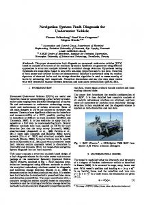
Figure 4. High Level Integrity Fault Tree for Loran

Two or More Cycles Incorrect

4. THE LORAN INTEGRITY FAULT TREE This section describes the current design of the Loran integrity fault tree and results to this date. Examination and quantification of the threats to Loran with respect to each requirement allow us to build the integrity fault tree. In the current fault tree, seen in Figure 4, we first divide the threats in two basic categories – Cycle Error and Phase/Timing Error (All Cycles Correct). Cycle errors are range errors that results from tracking the wrong cycle. Phase error results from the difference between the measured zero crossing and the actual zero crossing of the Loran carrier. We will consider timing and prediction errors as a subset of phase errors. 4.1 Loran Hazards Numerous threats can cause cycle error, phase error or both. This section enumerates the primary threats to cycle and phase. Many of these hazards were discussed in Section 2. For clarity, the threats to Loran are divided into three categories based on where the threats or issues exist or derive: from Loran transmitters, from propagation phenomena, and from the user receiver. The categories are seen in Figure 5.

Skywave Interference

• •

• Local Noise, P-static, Receiver Noise & Bias

Propagation Prediction Errors

Q

Figure 5. Threats to Loran Integrity Transmitter hazards to integrity include timing errors such as biases and jitter. Propagation hazards include ASF prediction errors. Errors in estimation of ASF result in timing errors. Hazards at the receiver include P-static, locally generated noise, atmospheric noise, sky wave and cross rate interference as well as receiver noise and biases. Atmospheric noise can cause significant phase error hence possibly resulting in integrity failure. Note that these threats are not exclusive to integrity. If the resulting error is too large and the receiver detects that it exceeds limits, the receiver may throw out the measurement resulting in loss of availability or continuity. 4.2 Cycle Errors

The primary cause of cycle error is Envelope to Cycle Differences (ECDs). ECD is the difference between the envelope TOA and the phase TOA. This error occurs because a Loran receiver first determines the TOA of the envelope. This envelope TOA is then used the select the nearest zero crossing, which determines the TOA used in the navigation solution. This is illustrated in Figure 6. If the total ECD error at the receiver exceeds one half cycle or 5 µsec, then a cycle error of 10 µsec occurs. The total ECD error at the receiver is the sum of:

•

Atmospheric Noise

Transmitter Bias& Jitter

Figure 6. Cycle and Phase Tracking

Transmitter ECD errors, (both bias and noise.) Errors in predicting the change in ECD as the signal propagates from transmitter to receiver (bias). Errors in the measurement due to noise and interference (both noise and bias) Errors in the calibration of the receiver (bias).

Since tracking the wrong cycle will result in a bias error that is an integer multiple of 10 µsec or 3000 meters, a HMI will occur if a measurement with an uncorrected and undetected cycle error is used in a position solution. Hence, cycle error dominates in this scenario regardless of phase error. The main issue associated with analytically proving Loran integrity is sufficient confidence in the correct cycle selection. Within the receiver, there is a cycle integrity monitor. Because of the importance of not using measurements with cycle errors, redundant information, when available, is used to form an over-determined position solution that allows for the calculation of cycle to a desired integrity. The basic cycle resolution algorithm is described in [5]. The implementation uses a calculated weighted sum square error (WSSE) statistic and a priori probabilities to determine the probability of being on a wrong cycle and not detecting the error, Pwc. A cycle slip or step detection algorithm is also used once the cycle has been initially validated. The LORIPP is currently finalizing the overall receiver cycle validation architecture. Figure 7 gives a sample architecture.

the probability that each error bound is not exceeded by its corresponding error. Finally, the fault tree divides the sources of error by where the error enters the Loran signal - transmitter, propagation prediction error, and interference at the receiver.

HPL = κ

∑ Kα i

i

Figure 7. Sample Receiver Architecture for Cycle Validation When the cycle resolution and step detection algorithms and the overall architecture are finalized, the LORIPP can determine the probability of the existence of one or more undetected cycle errors. The architecture will also determine the effects of the undetected cycle error relative to integrity and the probability that such an error will result in an HMI. For example, a low SNR station has a higher probability of having an undetected cycle error but the receiver algorithm may de-weigh or exclude measurement from this station due to its low SNR. These results are inputs to the integrity fault tree. 4.3 Phase Errors The probability of undetected cycle error should be very low. However, having no cycle error is not sufficient. Once a measurement is verified to be on the correct cycle, it still will contain phase and timing errors. The LORIPP will examine the characteristics of these errors and develop bounds consistent with meeting the integrity requirements. The analysis of each source of phase or timing error characterizes the error and builds an analytic model to bound the error. While the bound will be conservative, there is still a probability that the error will exceed the bound and hence a probability that the error will result in an HMI. This probability is then used in the integrity fault tree. Reduction of the HMI probability of each error depends on accurate characterization of the error. Each error characterized as one of three types and these types are explicitly laid out in the Loran Integrity Equation. 4.4 The Loran Integrity Equation The Integrity or HPL equation, Equation (1.1), characterizes phase errors into three forms. These forms are: 1) random, uncorrelated, and unbiased error, 2) completely correlated biases 3) uncorrelated biases. These bounds for these errors are denoted by the Greek letters α, β, γ, respectively. The true errors for each type are denoted as ε α, εβ , ε γ, respectively. If the phase error bounds are exceed by the actual errors, then there is a potential HMI. Hence, the fault tree examines

2 i

+

∑K β + ∑ K γ i

i

i

i i

(1.1)

i

Random, Uncorrelated and Unbiased Errors As a result of the properties of these errors, the confidence bounds for these errors can be root summed squared (RSS) together. Generally, α represents the one standard deviation level for an overbounding Gaussian distribution. So long as they are truly unbiased, and if εα i < αi , ∀ i , then the RSS bound will not be exceeded.

Completely Correlated Biased Since these errors are correlated, the confidence bounds for these errors can be added together before taking the absolute maximum. In other words, because of the correlation, we do not have to take the worst-case combination. Generally, β represents a not to exceed confidence level such as the 10-7 confidence level.

Uncorrelated Biased Since these errors are uncorrelated, the confidence bounds for these errors can be added together in the worst-case combination. Generally, γ represents a not to exceed confidence level such as the 10-7 confidence level.

The integrity fault tree utilizes this division of errors. Once each major integrity fault has been characterized and modeled, the probability of each type of error causing an integrity failure can be calculated. These probabilities are inputs for the integrity fault tree. The calculation can be treated in several ways. A conservative estimate is to assume that any time an error exceeds the bound, there is an integrity failure. Another method is to calculate the probability of exceeding the bound and then determine the probability exceeding the bound results in an HMI. 4.5 Example: Additional Secondary Factor (ASF) We will briefly discuss the ASF data collection and analysis as an example of the work that is being done. Residual difference between the true ASF and the applied ASF is one of the major sources of error. This task involves collecting data to determine values of ASF to provide to users and assess the residual errors after application of those ASFs. ASF values vary both temporally and spatially. In terms of temporal variations,

temporal and spatial variations of ASF. However, one year worth of data is not enough for integrity calculation and the analysis will be supplemented by other data. The USCG has digital data dating back many years. However, since the SAM control affected the timing, the data cannot be used directly. The effect of the SAMs can be eliminated using double differenced time difference (DDTD) though this limits the usefulness of the data.

ASF values have seasonal and daily variations caused by effects such as changes in surface refractivity and ground conductivity. A network of time of transmission (TOT) and time of arrival (TOA) monitors is currently being set up to collect data for this effort. TOT monitors are located at the Loran transmitters and TOA monitors are located at various user locations. These monitors allow for calculation of propagation times that are not adulterated by the control of the system area monitors (SAM) since the SAMs can shift the timing of the secondary Loran transmitters from the nominal transmission time. SAM control can thus mask the ASF.

Other data that may be examined is weather data. It has been observed that ASF variations are strongly correlated with the dry term of surface refractivity [6,7]. A model for ASF variations and level of variations can be built using the combination of TOT/TOA data and weather data. The ASF levels for previous years can be estimated using simulations. This will help determine bounds that can account for inter-year changes. Weather data thus can be used to supplement to collected ASF data. 4.6 Integrity Conclusions Data is currently being collected on the significant threats to integrity. Some of the data collection and analysis, such as ASF, will take a significant amount of time since year round data is required. Also data needs to be taken at many locations. Cycle integrity analysis depends both on the ECD data and analysis as well as the finalization of the cycle resolution and check algorithm. Once the data collection is finalized, then that section of the integrity analysis can be completed. The plan is to finish the integrity analysis by January 2004.

Figure 8. Time of Transmission (TOT)/Time of Arrival (TOA) Monitor Network TOT/TOA data will be collected for one year in various locations. This data will be used to identify and analysis

Continuity 99.9%

Loss of Signal

No Cycle Integrity

+

+

+

No Critical Transmitter

N or less Critical Transmitters

+

+

Two Transmitter Out

More than 2 Transmitter Out

+

+

Transmitter Off Air

Receiver Not Track

Transmitter Off Air

Transmitter Off Air

Fail Slip Detector

Receiver Not Track

Receiver Not Track

Figure 9. High Level Continuity Fault Tree for Loran

Fail RICC

5. CONTINUITY FAULT TREE Continuity is another major requirement that needs to be rigorously analyzed. As in the case with the integrity analysis, a hazard list and continuity fault tree was created to provide a thorough examination. The top level of the tree is divided into two means by which continuity is lost - loss of signal integrity (cycle integrity) or loss of signal.

Since there is redundancy built into the transmitter, equipment failure may not result in a loss of signal or it may result in only a temporary, i.e. three second, loss of signal. An analysis of transmitter set up and equipment failure rates is used to determine the availability and continuity of the transmitted signal. The signal generation path is shown in Figure 10.

5.2 Continuity Hazards While the hazards that affect continuity are often the same hazards that affect integrity, there are some differences. Transmitter hazards include transmitter outages due to equipment failures, operations, or transmitter monitors. While monitors at the transmitter ensure integrity by taking a station off air when it is out of tolerance, the outage may cause a loss of continuity and availability. Local interference threats are continuity hazards since they may result in loss of signal or loss of signal integrity. These include atmospheric noise, p static, local platform and receiver noise, sky wave interference and cross rate interference. Finally, other integrity threats such as ASF prediction error does not affect continuity. 5.3 Loss of Cycle Integrity Loss of cycle integrity on a signal is one reason why the signal from a normally available transmitter cannot be used. If the cycle integrity on at least three transmitters cannot be guaranteed in the middle of an approach, the approach must be terminated. The failure probabilities are dependent on the receiver architecture. However, there will be two primary ways of losing cycle integrity. First, a cycle step that cannot be corrected (if the cycle step detector fails and there is an uncorrectable step) will result in such an instance. Another possibility is if cycle resolution fails during an approach. Note that if cycle resolution fails at the beginning of an approach, the approach cannot be started and that is an availability issue. 5.4 Loss of Signal The other means for the user to lose Loran is for the receiver to not track a Loran signal. This can result from fault at the transmitter station or at the receiver.

Figure 10. LRP)

Loran Transmitter Signal Path (After

Statistical data on the duration of outages and time to repair for each component can then be used to determine the overall availability. Some of this data is deducible from manufacturers or historical records taken by the U.S. Coast Guard. Additional analysis and data is necessary to determine the Mean Time Between Failure (MTBF) and the mean time to repair (MTTR). MTBF is the reciprocal of the sum of the failure rates for all the component parts of the system. The availability and continuity of each component (over a 150 second period) is then given by:

5.4.1 Loss of Signal due to Transmitter The transmitter may be off air for numerous reasons – routine maintenance, transmitter equipment failure, etc.

MTBF =A MTTR + MTBF

(1.2)

MTBF − (150 − 1) =C MTBF

(1.3)

Availability = Continuity =

The transmitter signal generation model and failure probabilities of each component will be used determine the overall probability of transmitter failure. The probability of an available signal is the probability that there is at least one signal from the cesium to the antenna has not failed. Howe ver, failure of items such as the coupling networks (CN) or switch cabinet will require three seconds to switch to redundant circuitry. These momentary outages must also be taken into account. 5.4.1.1 Example: Transmitter Continuity Analysis We are currently completing the transmitter availability and continuity analysis. The analysis proceeds by determining two probabilities. Pin is the probability that, if the required input is available, the given component will yield an acceptable output. Pin is the same as the probability that the component is operating nominally. The second is Pout, the probability that a good input for the next piece of component has been generated by the specified component. For example, Pin for each cesium equals the probability that the cesium has not failed. Pout at the cesium is more difficult to calculate. There are three cesium clocks and the input to the timing frequency equipment (TFE) requires that at least two clocks are operating. For TFE 1, one of those clocks must be Cesium 1 and for TFE 2, one of those clocks must be Cesium 2. Pout for the Cesium 1 is equaled to the probability that Cesium 1 has not failed and either Cesium 2 or 3 has not failed.

probability that interference and noise can result in the loss of a signal. A model for the receiver operations will be created to determine the probability of the receiver not tracking a signal. 5.5 Relation between Loss of Signal and Loss of Continuity The loss of one Loran signal does not necessarily result in a loss of the Loran RNP 0.3 solution. Hence, there still may be availability and continuity even with the loss of one signal. In the case of one signal loss, we are concerned about critical transmitters. We define a “critical transmitter” as follows: If a given transmitter is required for all position solution that meets RNP 0.3 requirements, then the transmitter is critical. In other words, there are no solutions that meet requirements that do not require the measurement from a critical transmitter. Critical transmitters are determined by geometry. Since each location has a fixed geometry of transmitters, the continuity results are location dependent. For each location, we need to determine not only the number of critical transmitter but also the probability that a lost signal is from a critical transmitter. If there are no critical transmitters, two or more signals must be lost for a loss of continuity. The probability of two or more lost signals can be determined from the analyses of signal loss for the transmitter and receiver. Since the number of signals is location dependent, location will determine how many signals can be lost before there is loss of service/continuity. 5.6 Continuity Conclusions The LORIPP has now determined a methodology and formulated a fault tree for the continuity analysis. Work has begun on determining the availability and continuity figures necessary to complete the analysis. The transmitter continuity analysis is currently being completed and the receiver continuity analysis will begin once the receiver architecture has been agreed upon.

Figure 11. Transmitter Continuity Analysis (Cesium & TFE) 5.4.2 Loss of Signal at the Receiver The receiver may not track a Loran signal even though it is transmitted and has adequate signal strength. The loss may be due to interference (P-static, atmospheric noise) or receiver tracking issues. Analysis of the interference will provide some indication to the frequency and

6. CONCLUSIONS The LORIPP is progressing on its design and analysis of Loran for RNP 0.3 approaches. The integrity and continuity analysis are maturing. The fault tree for each requirement has laid out the overall analysis strategy. The tasks have now been divided into sections that are currently being examined. Results for both Loran RNP 0.3 integrity and continuity should be forthcoming within the following year.

REFERENCES [1] “Vulnerability Assessment of the Transportation Infrastructure Relying on the Global Positioning System,” John A. Volpe National Transportation System Center, August 20, 2001. [2] FAA (AND-700) report to DOT, An Analysis of Loran-C Performance, its Suitability for Aviation Use, and Potential System Enhancements, July 2002. [3] Weeks, G. K., Jr. and Campbell, M. “Status of the Loran Recapitalization Project (The Four Horsemen and TOC)”, Proceedings of the ION Annual Meeting, Albuquerque, NM, June 24-26, 2002. [4] Lo, S. et. al., “The Loran Integrity Performance Panel (LORIPP)”, Proceedings of the ION-GPS Meeting, Portland, Oregon, September 24-27, 2002. [5] Peterson, B. et. al., “Hazardously Misleading Information Analysis for Loran LNAV”, Proceedings of the International Symposium on Integration of LORANC/Eurofix and EGNOS/Galileo, DGON, June 2002. [6] DePalma, L. M. and Creamer, P. M., “Loran-C Grid Calibration Requirements for Aircraft Non-Precision Approach,” TASC Final Report for FAA, July 1982. [7] Sammaddar, S. N., "Weather Effect on Loran”, Navigation: The Journal of the Institute of Navigation, v. 27, no. 1, Spring 1980, pp. 39-53. DISCLAIMER -Note- The views expressed herein are those of the authors and are not to be construed as official or reflecting the views of the U.S. Federal Aviation Administration or Department of Transportation. ENDNOTES 1

Availability and continuity are expressed in a range of values from minimum to maximum. The “target” requirements listed in the table are derived from the U.S. standard for GPS that the Loran program is trying to achieve. The “minimum” requirements represent the ICAO standards that must be met. 2

The SAMs are fixed, unstaffed sites that continuously measure the characteristics of the Loran-C signal as received, detect any anomalies or out-of-tolerance conditions, and relay this information back to the control station so that any necessary corrective action can be taken. 99.9+% of the time the SAM “sees” no

abnormalities or out–of tolerance conditions, but provides measurements to allow (within tolerance) corrections to secondary transmission time and clock drift. Of the remaining < 0.1% of the time, the control station could take corrective action without the SAM another 99.9% of the time