LOW COMPLEXITY BAYESIAN SINGLE CHANNEL SOURCE SEPARATION Thomas Beierholm, Brian Dam Pedersen∗
Ole Winther†
GN ReSound A/S, M˚arkærvej 2A DK-2630 T˚astrup, Denmark
Informatics and Mathematical Modelling Technical University of Denmark, B321 DK-2800 Lyngby, Denmark
ABSTRACT We propose a simple Bayesian model for performing single channel speech separation using factorized source priors in a sliding window linearly transformed domain. Using a one dimensional mixture of Gaussians to model each band source leads to fast tractable inference for the source signals. Simulations with separation of a male and female speaker using priors trained on the same speakers show comparable performance with the blind separation approach of Jang and Lee [1] with a SNR improvement of 4.9 dB for both the male and female speaker. Mixing coefficients can be estimated quite precisely using ML-II, but the estimation is quite sensitive to the accuracy of the priors as opposed to the source separation quality for known mixing coefficients which is quite insensitive to the accuracy of the priors. Finally, we discuss how to improve our approach while keeping the complexity low using machine learning and CASA approaches [1, 2, 3, 4]. 1. INTRODUCTION Blind source separation is an active research subject within contemporary signal processing and machine learning. The blind separation of linearly mixed sources is possible because prior knowledge about the source signals is used. When the problem is well-determined, i.e. the number of sensors (channels) is at least as high as the number of sources, the source prior usually only needs to be quite weakly defined, e.g. in terms of their kurtosis, i.e. as sub-/super-Gaussian. The task of separating a mixture of sources in only one channel, on the other hand, requires strong prior knowledge. Together with the problem of separation of convolutive mixtures, this is the most interesting case seen from a hearing instrument industry point of view. Successful single channel speech separation are based upon building into the model strong prior knowledge. In the computational auditory scene analysis (CASA) this is achieved by hand crafting into the system knowledge about ∗ Email: † Email:
[email protected],
[email protected].
[email protected]
high level features of the speech signal such as pitch/periodicity and continuity [3, 4]. Machine learning methods can also be used to extract such features by training e.g. hidden Markov models (HMM) on speech periodograms for single speakers [2]. These HMM work as priors for the sources in the single channel mixed signal. Independent component analysis can be used to extract basis filters and priors in a sliding window based approach [1]. The basis filters and associated independent source priors in the transformed domain exploits the underlying probabilistic characteristics of the speech signals. Our approach is familiar in spirit with Ref. [1]. We make the simplifying assumption that both speakers share basis filters which for simplicity here is chosen to be discrete cosine transforms (DCT). Using a mixture of Gaussians prior, we furthermore keep all inference tractable such that we can use a Bayesian estimator for the sources as opposed to the maximum likelihood (ML) approach used in Ref. [1]. These simplifying assumptions has been used because it has been the motivation for the work presented in this paper to keep the analysis simple and computational complexity as low as possible while achieving separation comparable to e.g. Ref. [1]. 2. SOURCE SEPARATION MODEL The single channel two sources separation problem can be expressed in the following way: The mixture xt is assumed to be an instantaneous linear broad band mixture of two independent sources st1 and st2 xt = λ1 st1 + λ2 st2 + η t ,
(1)
where the sources have been weighted with time invariant mixing coefficients λ1 and λ2 and noise has been added to the mixture. Independence of the sources can be expressed simply as a factorization of the joint distribution of the signals: p({st1 }, {st2 }) = p({st1 })p({st2 }). The basic idea of the approach examined in this paper is to build a probabilistic model for sources in some linear transformed domain and perform the separation of the sources in each band assuming complete independence over
time and bands. In this way we achieve simple analytically tractable inference while we by using block based processing exploit temporal correlation inherent in speech signals. Mathematically, the transformed domain variables can be expressed as ˆ (t) = (ˆ x x1 (t), . . . , x ˆN (t))T = F [x(t)] ,
(2)
where x(t) = (xt , xt+1 , . . . , xt+(N −1) )T is the tth sample window vector and the band index runs from 1 to the blocksize N . We will also assume that the inverse F −1 exists. In the next section we will discuss the specific choice of F in this work and in the literature. Due to the linearity of the transform, eq. (1) turns into an identical eq. in the transˆ (t) = λ1 ˆs1 (t) + λ2ˆs2 (t) + η ˆ (t). The cruformed domain: x cial assumption for making a low complexity algorithm is that the joint distribution of the transformed variables over Q time and bands factorizes, i.e. p({ˆsm (t)}) = it p(ˆ sim (t)) with source index m = 1, 2. Ideally the transform will be chosen such that each band represent independent features. Clearly, the bands are very correlated for nearby times since there will be a big overlap of the windows used to calculate the transformed sources. The block based representation introduces redundancy in the estimation, i.e. once we have obtained estimates of the sources ˆsest m (t), we get N estimates of each source signal stm from the inverse transformations ˜ ˜ F −1 [ˆsest m (t)], t = t − (N − 1), . . . , t. An empirical investigation shows that these N estimates are rather consistent, i.e. their standard deviation is somewhat smaller than typical deviation from the true source value. This justifies using the mean over the N estimates as the final estimator. Next, we will go through the Bayesian estimation theory for the source signals. Since we have assumed complete independence we can omit all time and band indices and write the posterior distribution of the specific source as p(ˆ s1 , sˆ2 |ˆ x , λ 1 , λ2 ) =
p(ˆ x|ˆ s1 , sˆ2 , λ1 , λ2 )p(ˆ s1 )p(ˆ s2 ) , (3) p(ˆ x|λ1 , λ2 )
where the normalizing factor Z p(ˆ x|λ1 , λ2 ) = dˆ s1 dˆ s2 p(ˆ x|ˆ s1 , sˆ2 , λ1 , λ2 )p(ˆ s1 )p(ˆ s2 ) is the likelihood for the λs for that specific sample. The likelihood p(ˆ x|ˆ s1 , sˆ2 , λ1 , λ2 ) expresses our observation model, i.e. for Gaussian noise we have log p(ˆ x|ˆ s1 , sˆ2 , λ1 , λ2 ) ∝ − 2ˆσ1 2 (ˆ x − λ1 sˆ1 − λ2 sˆ2 )2 , where σ ˆ 2 is the noise variance. In section 4 we will discuss how to choose and tune the prior distribution for the speakers we want to separate. Although we need very precise prior knowledge tuned to the specific speaker to perform source separation in this underdetermined case, we can still estimate the mixing coefficients blindly. This will be done by maximum likelihood II. Since we have assumed independence, the likelihood is
a product over bands and time and we get X log p(ˆ xi (t)|λ1 , λ2 ) λm = argmax λm
(4)
it
Finally, we will use the posterior mean (Bayes optimal for square loss) as the estimator for the sources: sˆest sm i ≡ m = hˆ R sˆm p(ˆ sm |ˆ x, λ1 , λ2 ) dˆ sm . 3. TRANSFORMED DOMAIN An important question is what transform to use. Obviously, the ideal choice is one which make sources in the different bands statistically independent. Because then at least our assumption of independence over bands at one time instant is correct. Here we have chosen the Discrete Cosine Transform (DCT) due to the following properties of the DCT: its unitary, its real and its robust to noise on the transform coefficients. The DCT is unitary meaning that there is no information lost in going from the time domain to the transform domain and it means that the transform is orthogonal and hence have a decorrelating effect on the transform coefficients. The DCT is real which besides making it relatively fast to compute also alleviates problems that would otherwise occur if we had chosen to use the DFT (or other complex transform) such as time aliasing, reuse of ’noisy’ phases, increased sensitivity to noise on the coefficients and complications in the probabilistic description. The disadvantage of the DCT is that the sources in the transformed domain are not independent which is easy to see if other statistics than the first and second order are calculated. Jang and Lee [1] use a set of basis filters Am , m = 1, 2 and associated priors that are learned from data such that the sources ˆsm are independent. Their generative model is thus stm = Amˆsm (t) and xt = λ1 st1 +λ2 st2 . Multiplying xt with t ˆ (t) ≡ A−1 s2 (t). s1 (t) + λ2 A−1 A−1 1 A2 ˆ 1 , we get x 1 x = λ1 ˆ Now if either A1 = A2 by construction or there exists a suitable permutation matrix P, P2 = I, such that that A−1 1 A2 P is nearly diagonal then we can use the framework developed above directly on ˆs1 (t) and Pˆs2 (t) with mixing coefficients λ1 and λ2 diag(A−1 1 A2 P). This will be tested in a future publication. 4. ESTIMATING THE PRIOR DCT coefficients were extracted from a male and a female speech signal obtained from Ref. [1] and the resulting histograms plotted as illustrated in figure 1. As can be seen in this example the distribution is sharply peaked around zero and show long-tailed tendencies and this applies for all bands. We therefore choose to model the distribution with a zero mean mixture of Gaussians (MoG) X p(ˆ s) = πk Nsˆ(0, σk2 ) , (5) k
P 6. RESULTS AND EVALUATION where the mixing proportions πk are normalized to 1: k πk = 1 and Nz (µ, σ 2 ) is the 1D Gaussian distribution for z with In estimating the mixing coefficients it was found that the mean µ and variance σ 2 . Maximum Likelihood estimation fit of the prior distribution to the actual (true) distribution is of the parameters can be done with the EM algorithm. We crucial. For the case of using Laplacian priors and speech also fitted a Laplacian prior p(ˆ s) = α2 exp(−α|ˆ s|). The resignals the estimated mixing coefficients were so much off sults of the fit can also be seen in the figure 1. All the MoG that the Laplacian prior was found useless. When using synmodels make pretty good fits. However, the Laplacian, even thetic generated Laplacian distributed signals, mixing coefthough suggested as a good speech model [5], is too unflexficients could be determined very accurately, but for speech ible for both fitting the peak and the tails. signals it was impossible to get any accuracy at all. For Comparison of distributions and fit to speech DCT coefficient the MoG prior, the accuracy of the estimated mixing coefx 10 4 ficients when increasing the number of components in the 0.025 Speech mixture is improved and this further supported our point 3.5 laplacian ML 3 mixture gaussian that the fit of the prior is important in estimating the mix0.02 4 mixture gaussian 5 mixture gaussian ing coefficients. For the case of mixing two speech signals 3 (each 1 second long sampled @ 16kHz) with mixing coef0.015 ficients λ = 0.3 and λ2 = 0.7 the estimated mixing co2.5 1 = efficients for 2 to 5 components MOG priors were λML 1 0.01 2 = (0.788, 0.727, (0.186, 0.249, 0.258, 0.263) and λML 2 0.715, 0.709). 0.005 1.5 An experiment was conducted where separation was performed on male and female speech segments (2 seconds 0 −0.5 −0.4 −0.3 −0.2 −0.1 0 0.1 0.2 0.3 0.4 0.5 1 DCT band value [magnitude] long with λ1 = λ2 = 1) obtained from Ref. [1]. This test showed that given a high enough DCT resolution (N=256) 0.5 and perfect knowledge about the MoG parameters (4 components were used) a signal-to-noise ratio improvement of 0 0.5 1 1.5 2 2.5 3 4.9 dB for both the male and female speech were obtained. DCT band value [magnitude] The SNR improvement is computed as difference in SNR after separation and before separation (in bands), where the Fig. 1. Fit of priors to observed data for 10th band male noise in the separated signals is estimated as the original speaker. speech minus the estimated speech. The SNR improvement over bands can be seen in figure 2. In Ref. [1] better separation at the expense of severe artifacts is obtained whereas our approach obtains less separa5. BAYESIAN INFERENCE IN MIXTURE OF tion but has virtually no audible artifacts. The resulting SNR GAUSSIANS improvements are the equal. All relevant sound samples include for comparison those from Ref. [1] are available at Using an additive Gaussian noise observation model and the isp.imm.dtu.dk/staff/winther/. MoG priors we can derive analytically tractable expressions The attenuation of the secondary source is getting more for the likelihood and the posterior mean estimator: profound the larger the block size used and the more the KX prior distributions of the sources differ. The approach nat1 ,K2 urally works better the more separated the sources are in πk1 πk2 Nxˆ (0, σk21 k2 ) p(ˆ x|λ1 , λ2 ) = frequency. For the sounds used in the evaluation no audik1 ,k2 ble artifacts or distortion was introduced in the estimated sources. KX 1 ,K2 2 λm σ x ˆ hˆ sm i = πk1 πk2 2 km Nxˆ (0, σk21 k2 ) , p(ˆ x|λ1 , λ2 ) σk 1 k 2 7. DISCUSSION AND OUTLOOK −3
k1 ,k2
where we for simplicity have set the noise variance to zero, omitted band and time indices and defined σk21 k2 ≡ λ21 σk21 + λ22 σk22 . It is interesting to note that the estimator reduces to the Wiener filter for K1 = K2 = 1 widely used in classical signal processing methods and speech enhancement.
The approach we have taken shows SNR improvement in separating a single channel mixture of one male and one female speaker. This improvement is gained in ideal conditions, but also with modest utilization of prior knowledge in the respect that we make a very fine tuned model of the
Estimated male
60
7
6
6
6
50
5
40
5 4 3 2
Frequency [kHz]
7
5 4 3 2
4
1
0
0
0
1 1.5 Time [s]
2
6
Frequency [kHz]
7
6 5 4 3 2
2
0.5
1 1.5 Time [s]
2
10 5
4
0
3 −5
2 1
0
0
2
10
SNR improvement [dB]
5
1 1 1.5 Time [s]
1 1.5 Time [s]
Estimated female
7
0.5
0.5
20
2
1 0.5
30
3
1
Original female
Frequency [kHz]
Mixture
7 Frequency [kHz]
Frequency [kHz]
Original male
−10 0.5
1 1.5 Time [s]
2
Male Female 0 1 2 3 4 5 6 7 8 Frequency [kHz]
Fig. 2. Spectrograms for original, mixed and separated signals. SNR improvement as a function of frequency.
statistical properties of single bands in the sliding window based approach, but use no prior knowledge about the speech signal and the human auditory system such as pitch/periodicity, redundancy, temporal correlation, effects related to psychoacoustics, etc. We believe that large improvements can be obtained if the temporal and spectral correlations in speech signals are used. The approach we have taken uses temporal information only implicitly in going to the transformed domain, but does not exploit spectral correlation at all. The advantage of our simplistic approach is that since we ignore all correlations, i.e. model the sources in the transformed domain as independent, we can make fast exact Bayesian inference using a mixture of Gaussians (MoG) prior. Future extensions should be aimed at utilizing spectral and temporal information as much as possible and fit it into the Bayesian framework while keeping the model simple. This will be discussed below. Our approach resembles the approach of Jang and Lee [1]. The differences are that they use a different transform (actually learned from data), a different family of priors (called generalized Gaussians) and due to non-tractability estimate the sources using maximum likelihood and not by Bayesian inference. The transform and the priors are designed to make the sources statistically independent which of course is also what we ideally are after. A listening test and calculation of SNR improvements show that the two approaches give similar performance. We expect that an improvement in performance can be obtained by using a learned transform while retaining the assumption of independence to keep the method analytical tractable. The excellent results of the CASA [3, 4] and Roweis’ CASA inspired machine learning approach [2] show that it
is important to model higher level speech features such as pitch detection/tracking. The CASA approaches relies on a 0/1-masking of the bands to perform separation. When we turn our Bayesian estimator into a masking function (by dividing the variances of the mixture components by the same large number) we find a decreased performance. This suggests that masking at least in our approach is not ideal and that it is worthwhile to combine higher level features with the Bayesian estimation of the single bands. In the following we will outline a simple low complexity approach to this, taking the pitch (fundamental frequency) as an example of a high level feature. First we extract the fundamental frequencies of a signal (marginalizing over the number of harmonics), i.e. we get the distribution of the set of fundamental frequencies fˆ1 , fˆ2 , . . . in the given windowed signal x: p(fˆ1 , fˆ2 , . . . |x). If we can assign a funt damental frequency to each speaker, fm , m = 1, 2, we can build source priors that are conditioned on the fundament tal frequency, i.e. p(ˆ si (t)|fm ) that can be used directly in t the framework presented in the paper. To infer fm , we can use the above mentioned extraction method on the unmixed t signals to build a (Markov) model for each speaker: p(fm ) t t−1 t and p(fm |fm ). We can now infer fm , m = 1, 2 from the extracted frequencies (assuming two extracted Q frequencies): t t−1 t t−1 t |fm ) p({fm }|fˆ1t , fˆ2t , {fm }) ∝ p(fˆ1 , fˆ2 |{fˆm }) m,t p(fm and the likelihood with equal assignment prob. becomes t p(fˆ1 , fˆ2 |{fm }) = 12 (p(fˆ1t |f1t )p(fˆ2t |f2t )+p(fˆ1t |f2t )p(fˆ2t |f1t )). We expect that enhanced performance can be achieved by extracting a statistically decorrelating set of basis filters [1] in combination with simple models of high level speech features. We are currently pursuing this with the aim of building low complexity single channel source separation with state-of-the-art performance. 8. REFERENCES [1] G.-J. Jang and T.-W. Lee, “A probabilistic approach to single channel blind signal separation,” in NIPS. 2003, vol. 15, MIT Press, speech.kaist.ac.kr/∼jangbal/. [2] S. T. Roweis, “One microphone source separation,” in NIPS. 2001, vol. 13, pp. 793–799, MIT Press. [3] D. L. Wang and G. J. Brown, “Separation of speech from interfering sounds using oscillatory correlation,” IEEE Trans. Neural Networks, vol. 10, pp. 684–697, 1999. [4] G. Hu and D. Wang, “Monaural speech separation,” in NIPS. 2003, vol. 15, pp. 1221–1228, MIT Press. [5] S. Gazor and W. Zhang, “A soft voice activity detector based on a laplacian-gaussian model,” IEEE trans. speech and audio processing, vol. 11, 2003.