Recursive Update Algorithm for Iterative ..... stated in the following optimization problem: minimize E|xi(k) ... It can be shown that the optimal solution [6], [8]â[10] is given by, .... complexity reduction since it costs nothing to iterate from. P(nâ1).
Low Complexity Linear MMSE detector with Recursive Update Algorithm for Iterative Detection-Decoding MIMO OFDM system Daniel N. Liu and Michael P. Fitz Department of Electrical Engineering University of California Los Angeles, Los Angeles, CA, 90095 Email: {daniell and fitz}@ee.ucla.edu Abstract— Iterative turbo processing between detection and decoding shows near-capacity performance on a multiple-antenna system. Combining iterative processing with optimum frontend detection is particularly challenging because the front-end maximum a posteriori (MAP) algorithm has a computational complexity that is exponential in the throughput. Sub-optimum detector such as the soft interference cancellation linear minimum mean square error (SIC-LMMSE) detector with near frontend MAP performance has been proposed. The asymptotic computational complexity of SIC-LMMSE remains O(n2t nr + nt n3r + nt Mc 2Mc ) per detection-decoding cycle where nt is number of transmit antenna, nr is number of receive antenna, and Mc is modulation size. A lower complexity detector is the hard interference cancellation LMMSE (HIC-LMMSE) detector. HIC-LMMSE has asymptotic complexity of O(n2t nr + nt Mc 2Mc ) but suffers extra performance degradation. In this paper, we introduce a low complexity front-end detection algorithm that not only achieves asymptotic computational complexity of O(n2t nr + nt n2r [Γ (β) + 1] + nt Mc 2Mc ) where Γ (β) is a function with discrete output {−1, 2, 3, ..., nt }. Simulation results demonstrate that the proposed low complexity detection algorithm offers exactly same performance as its full complexity counterpart in an iterative receiver while being computational more efficient.
I. I NTRODUCTION Ever since Berrou and Glavieux published their landmark paper on iterative decoding between two parallel concatenated convolutional codes (turbo-codes) [1], [2], it has been generally accepted that iterative (turbo) processing techniques have great value. As pointed out in [3] the “Turbo Principle” not only can be used with traditional concatenated channel coding schemes, but also generally applies to many detectiondecoding algorithms. Of late, multiple-input multiple-output (MIMO) systems receive tremendous amount of attention due to the information theoretic studies done by Telatar, Foschini and Gans [4], [5]. To approach channel capacity in a computationally efficient manner, it seems quite natural to apply the “Iterative(Turbo) Paradigm” to MIMO systems. Therefore, many of iterative detection-decoding algorithms have successfully been generalized to MIMO enviroment [6]–[8], especially multiple-input multiple-output orthogonal frequency division multiplexing (MIMO-OFDM) systems [9]. The complexity of optimum front-end MIMO detection motivates the search for a low complexity suboptimal detector. In fact, the optimal front-end MAP detector has complexity that grows exponentially with the modulation size and the
number of antennas. To address complexity issues, suboptimal detectors/decoders such as: soft interference cancellation linear minimum mean square error (SIC-LMMSE) detector [6], [9], [10], hard interference cancellation LMMSE (HIC-LMMSE) detector [8], [11] and “list” sphere decoder [12] are proposed in the literature. However, the asymptotic computational complexity of this SIC-LMMSE detector is O(n2t nr + nt n3r + nt Mc 2Mc ) per detection-decoding cycle (i.e. turbo iteration) [8], [13], where nt is number of transmit antenna, nr is number of receive antenna and Mc is modulation size. Despite the SIC-LMMSE detector having a linear growth in the number of transmit antennas, it’s computational complexity remains high even with moderate number of nt , nr and Mc . Further reduced complexity detection such as the HIC-LMMSE detector is also advocated in [8], [11]. HIC-LMMSE has asymptotic computational complexity of O(n2t nr +nt Mc 2Mc ) at the price of performance degradation. By reformulating a matrix inversion step in SIC-LMMSE detection algorithm into Recursive Update Algorithm (RUA), SIC-LMMSE detector is transformed into a structure more suitable for iterative detection and decoding receiver. In particular, SIC-LMMSE detector with RUA allocates its computational power depending on the level of the a priori information provided by outer channel decoder. As number of turbo iteration increases, a priori information becomes more and more reliable. Thus, asymptotic complexity of O(n2t nr + nt n2r [Γ (β) + 1] + nt Mc 2Mc ) is achieved without any performance degradation, where Γ (β) is a function with discrete output {−1, 2, 3, ..., nt }. The remainder of the paper is organized as follows: Section II presents the system model and introduces our notation. Section III introduces the SIC-LMMSE with RUA detector. Section IV presents several numerical examples for different number of receive and transmit antennas on standard wireless local area network (WLAN) channel model. Section V concludes the paper. II. S YSTEM M ODEL A. Transmitter We consider a multiple-input multiple-output orthogonal frequency division multiplexing (MIMO-OFDM) system with nt transmit and nr receive antennas. The transmission scheme
850 U.S. Government work not protected by U.S. copyright This full text paper was peer reviewed at the direction of IEEE Communications Society subject matter experts for publication in the WCNC 2006 proceedings.
GI insertion
x1 (k)
IFFT
mapper µ S/P
MIMO channel H(k)
AWGN
AWGN
GI insertion
IFFT
GI removal n(k)
FFT
GI removal n(k) Fig. 1.
xnt (k)
nr ×nt
b
LDPC encoder
mapper µ
LA
y1 (k) MIMO detector
LE
LDPC decoder
ˆ b
ynr (k)
FFT
Iterative detection-decoding MIMO-OFDM system
is detailed in the upper half of Fig. 1. Let vector b with size Nb be source information bits entering the rate Rc LDPC channel encoder. We denote c the vector of encoded bits; which is not only grouped into blocks of Mc bits where Mc is number of bits per constellation symbol, but also multiplexed to nt sub-streams. We will consider a linear model at the kth frequency subcarrier in which received vector y(k) = T [y1 (k), . . . , ynr (k)] ∈ Cnr ×1 depends on transmitted vector T x(k) = [x1 (k), . . . , xnt (k)] ∈ Cnt ×1 via y(k) = H(k)x(k) + n(k)
c
(1)
is complex channel matrix, known where H(k) ∈ C perfectly by receiver, n(k) ∈ Cnr ×1 is a vector of independent zero-mean complex Gaussian noise entries with variance σ 2 = N0 /2 per each real component and k = 1, 2, . . . , K where K refers to total number of frequency subcarriers. We assume the average symbol energy Es ≡ E|xi (k)|2 = 1 where i = 1, 2, . . . , nt and symbols are equally likely chosen from a complex constellation X with cardinality |X | = 2Mc . The spectral efficiency R is then defined as R = nt Mc Rc bits per channel use (BPCU). We also define the signal-to-noise ratio (SNR) as Eb /N0 , where Eb is the energy per transmitted information bit per receive antenna. Notice that each receive antenna collects total energy of nt Es which carries nt Mc Rc information bits, therefore Eb can be expressed as Eb = Es /(Mc Rc ). We assume that the data model (1) is used repeatedly for each frequency subcarrier k to transmit a continuous stream of information bits. During each application of data model (1), the channel matrix H(k) is a “snapshot” of the frequency response of MIMO propagation channel between all transmit and receive antennas. More specifically, H(k) is fully described as � � (2) H(k) = h1 (k) h2 (k) · · · hnt (k)
T
where hi (k) = [h1,i (k), h2,i (k), . . . , hnr ,i (k)] and hj,i (k) represents the complex channel coefficient from transmit antenna i to receive antenna j, j = 1, 2, . . . , nr , at kth frequency subcarrier. B. Iterative Receiver Structure The iterative receiver structure is depicted in the lower half of Fig. 1. The MIMO detector takes the channel observation y(k) and a priori log-likelihood ratio (LLR) LA (cl ) to compute the extrinsic information LE (cl ) for each of nt Mc bits per received vector y(k). With cl = +1 representing a binary one and cl = −1 representing a binary zero, we define LA (cl ) from outer channel decoder as LA (cl ) ≡ log
P [cl = +1] P [cl = −1]
(3)
where l = 1, . . . , nt Mc . Moreover, LA (cl ) can also be viewed as the extrinsic information learned at the outer channel decoder. The a posteriori LLR LD (cl |y(k)) for bit cl , conditioned on received vector y(k) is similarly defined as LD (cl |y(k)) ≡ log
P [cl = +1|y(k)] P [cl = −1|y(k)]
(4)
where P [cl = m|y(k)], m = ±1, is the a posteriori probability (APP) of bit cl . Using Bayes’ theorem, (4) can be rewritten as LD (cl |y(k))
P [cl = +1] P [y(k)|cl = +1] + log P [y(k)|cl = −1] P [cl = −1] (5) = LE (cl ) + LA (cl ) = log
where the first term in (5), denoted as LE (cl ), is the extrinsic information delivered by MIMO detector, based on the received vector y(k) and prior information about the coded bits LA (cl ). “New” (extrinsic) information learned at the detection
851 This full text paper was peer reviewed at the direction of IEEE Communications Society subject matter experts for publication in the WCNC 2006 proceedings.
stage can easily be separated from a posteriori LLR LD (cl ) by subtracting off the a priori LLR LA (cl ). That is, LE (cl ) = LD (cl |y(k)) − LA (cl ).
(6)
In view of (6), extrinsic information LE (cl ) is then fed into outer channel decoder as a priori information on the coded bit cl . III. SIC-LMMSE D ETECTOR WITH RUA As a priori LLR becomes available, we form symbol mean x ¯i (k), i = 1, 2, . . . , nt , as � x ¯i (k) = xP [xi (k) = x], (7) x∈X
where X is the complex constellation set and P [xi (k) = x] refers to a priori symbol probability. Assuming bits within symbol x are statistical independent and let x˜l represents the ˜lth bit value of symbol x (i.e. x˜ = +1 means ˜lth bit of symbol l x is binary one), where ˜l = 1, 2, . . . , Mc , then P [xi (k) = x] can be computed as P [xi (k) = x] =
Mc � ˜ l=1
1 . 1 + e−xl˜LA (cl˜)
(8)
For ith transmit antenna, interference from rest of nt − 1 antennas is “parallel” cancelled to obtain yi (k) nt �
= y(k) −
x ¯n (k)hn (k)
n=1,n�=i
= xi (k)hi (k) +
nt �
(xn (k) − x ¯n (k))hn (k) + n(k).
n=1,n�=i
(9) The LMMSE filter wi (k) is chosen to minimize the meansquare error (MSE) between the transmit symbol xi (k) and the filter output x ˆi (k). Equivalently, LMMSE filtering is precisely stated in the following optimization problem: minimize E|xi (k) − x ˆi (k)|2 subject to x ˆi (k) = wi (k)† yi (k),
where the covariance matrix ∆i (k) is �
= diag
σx21 (k) Es
,··· ,
σx2i−1 (k) Es
, 1,
x∈X
In view of (11), the LMMSE filter adapts its filter coefficients according to the quality of soft interference cancelled symbols through covariance matrix ∆i (k). Depending on the level of a priori LLR LA (c˜l ), actual value of symbol variance σx2i (k) can range from zero to Es . Hence, small symbol variance ¯i (k), approaches the σx2i (k) indicates that symbol mean, x true transmit symbol xi (k) and soft interference cancellation perform in (9) is near perfect. There is an interesting way to perform matrix inversion via a recursive update algorithm (RUA). As (11) suggests, finding the optimal LMMSE filter coefficient wi (k) often involves solving a system of equations which is also the most “expensive” step in the algorithm in terms of complexity. Efficient methods such as QR decomposition and Cholesky factorization [14] are used in practice for solving such system of equations, but still at the cost of cubic complexity [14]. One na¨ıve way to “solve” the system of equations would be inverting a nr × nr matrix of � �−1 N0 † Pi (k) = In + H(k)∆i (k)H(k) , (14) Es r and compute wi (k) = Pi (k)hi (k). In what follows, we will propose an algorithm to construct Pi (k) directly via recursive update. A similar idea can also be found in [10] for multiuser detection. We define the following matrices
−1 nt −1 2 σxn (k) Es � (nt −1) † Pi (k) = Inr + hn hn , (15) N0 n=1 Es
−1 nt σx2n (k) Es � (nt ) † hn hn . (16) Pi (k) = Inr + N0 n=1 Es We then can rewrite the term H(k)∆i (k)H(k)† in (14) as sum of vector outer products
(10)
where (·)† denotes conjugate-transpose. Hence, the optimal LMMSE filter coefficient wi (k) is obtained by solving (10). It can be shown that the optimal solution [6], [8]–[10] is given by, � �−1 N0 Inr + H(k)∆i (k)H(k)† hi (k), (11) wi (k) = Es ∆i (k)
and σx2n (k) , n = 1, 2, . . . , nt with n �= i, is the transmit symbol variance and generally can be computed as, � σx2i (k) = |x − x ¯i (k)|2 P [xi (k) = x]. (13)
H(k)∆i (k)H(k)† =
nt � σx2n (k) n=1
Es
hn h†n .
(17)
In view of (17), we can re-express (14) as
−1 nt σx2n (k) Es Es � † Pi (k) = hn hn Inr + N0 N0 n=1 Es =
Es (nt ) P (k). N0 i
(18) (n )
σx2i+1 (k) Es
,··· ,
σx2n
� t (k)
Es
,
(12)
The recursive update relation hinges on rewriting Pi t (k) as shown in (19). To arrive at (19), we had applied the “degenerate” matrix inversion lemma [14]. As (19) suggests, (n −1) we have found a recursive update relation between Pi t (k) (nt ) and Pi (k). Therefore, we can directly construct Pi (k) by RUA which is outlined in Table I.
852 This full text paper was peer reviewed at the direction of IEEE Communications Society subject matter experts for publication in the WCNC 2006 proceedings.
(n ) Pi t (k)
=
(n −1) Pi t (k)
2 σx n
−
1+
2 σx nt (k)
N0
t (k)
N0
�
(nt −1)
h†nt Pi
TABLE I R ECURSIVE U PDATE A LGORITHM
(k)hnt
� † � (nt −1) (n −1) (k)hnt Pi t (k)hnt Pi
the value selected for β (i.e. β = 0), less likely that Pi (k) will be formed in exactly one iteration, which implies more computational complexity. On the other hand, a larger value of β (i.e. β = 1) will be more likely to form Pi (k) in exactly one iteration (i.e. HIC-LMMSE detection). The output of LMMSE filter is,
(0)
1. Initialization: Pi (k) = Inr . for n = 1, 2, . . . , nt (n) (n−1) 2. Updating Pi (k) from Pi (k) as shown in (19). end Es (nt ) 3. Pi (k) = N Pi (k). 0
Because of this recursive algorithm the detection problem on the MIMO channel can be transformed into a structure more suitable for iterative detection and decoding receiver. Conventionally, SIC-LMMSE detector forms its optimum LMMSE filter coefficient wi (k) by solving system of equations without incorporating a priori information. Thus, fixed amount of computational resources are allocated uniformly through out the iterative detection-decoding process. Different from SICLMMSE detector, SIC-LMMSE detector with RUA obtains wi (k) by directly constructing Pi (k) which is made explicitly a function of a priori information. Without a priori information, RUA is still a cubic complexity algorithm to form Pi (k). (n) But, once a priori information becomes available, Pi (k) is (n−1) only updated from the previous iteration Pi (k) in (19) when σx2n (k) /N0 � 0, n �= i, where σx2n (k) is computed from a priori LLR. Hence, SIC-LMMSE detector with RUA enables a more flexible allocation of computing power depending on the level of a priori information. The RUA is mainly a function of “effective” signal-to-noise ratio, SNRe (n), SNRe (n) =
σx2n (k)
, n �= i,
(19)
x ˆi (k) = µi (k)xi (k) + zi (k),
(21)
µi (k) = wi (k)† hi (k),
(22)
where
and zi (k) is the ISI-plus-noise term. As shown in [15], we approximate x ˆi (k) the output of LMMSE filter as complex Gaussian distributed given xi (k). That is, P [ˆ xi (k)|xi (k) = x] ∼ Nc (µi (k)x, ηi2 (k)) − 21 |ˆ xi (k)−µi (k)x|2 1 = e ηi (k) , 2 πηi (k) where x ∈ X and the variance ηi2 (k) is given by, ηi2 (k) = (µi (k) − µ2i (k))Es .
N0 which also appears in (19). Depending on the number of turbo iterations and Eb /N0 , the actual value of SNRe (n) is varying. If SNRe (n) < β, where β is the threshold, the RUA skips the updating step as in (19) and achieves a lower complexity. In particular, since a priori LLR becomes more and more reliable as the number of turbo iteration increases, the “estimated” symbol mean x ¯i (k) becomes more likely to be the true transmit symbol while the “estimated” symbol variance σx2n (k) , n �= i, is approaching zero. When σx2n (k) = 0, n �= i, (i.e. perfect cancellation), RUA achieves further complexity reduction since it costs nothing to iterate from (n−1) (n) (k) to Pi (k) with n �= i as clearly shown in (19). Pi Thus, Pi (k) is formed exactly one iteration at n = i which in effect forms MRC filter with the corresponding column vector hn of channel matrix. The explicit parameterization of threshold β in SICLMMSE detector with RUA enables a trade-off between achieving a lower complexity and better performance. Smaller
(24)
Having (8) and (23) in mind, the a posteriori LLR xi (k)), ˜l = 1, 2, . . . , Mc , is computed for each detecLD (c˜l |ˆ tion symbol estimate x ˆi (k) (i.e. i = 1, 2, . . . , nt ) per transmit T ˆ (k), where x ˆ (k) = [ˆ antenna within x x1 (k), . . . , x ˆnt (k)] via, xi (k)) LD (c˜l |ˆ
= log
x∈X˜+1
P [ˆ xi (k)|xi (k) = x] P [xi (k) = x]
x∈X˜−1
P [ˆ xi (k)|xi (k) = x] P [xi (k) = x]
l
l
(20)
(23)
,
(25)
where X˜l+1 is the set of 2Mc actual constellation symbols x which the ˜lth bit is +1 (i.e. x˜l = +1). With (25), SIC-LMMSE detector computes the extrinsic LLR LE (c˜l ) as, xi (k)) − LA (c˜l ). LE (c˜l ) = LD (c˜l |ˆ
(26)
Replacing original matrix inversion with RUA in SICLMMSE detector will allow a more efficient computation of detection symbol estimate as number of turbo iteration increases. When a priori information feedback from outer channel decoder becomes very reliable, SIC-LMMSE detector with RUA forms its detection estimate x ˆi (k) via MRC filter which is same as HIC-LMMSE detector. On the other hand, unlike HIC-LMMSE detector which always uses MRC filter, SIC-LMMSE detector with RUA also utilizes “unreliable” a priori information to form x ˆi (k) as clearly shown in (19). Table II gives a detailed outline of SIC-LMMSE detector with RUA. At the first turbo iteration, SIC-LMMSE detector with RUA share the same computational complexity as SIC-LMMSE detection algorithm which is O(n2t nr + n3r +
853 This full text paper was peer reviewed at the direction of IEEE Communications Society subject matter experts for publication in the WCNC 2006 proceedings.
TABLE II SIC-LMMSE DETECTION ALGORITHM WITH RUA
0
10
for i = 1, 2, . . . , nt 1. Find a priori symbol probability P [xi (k) = x] as in (8). 2. Find symbol mean x ¯i (k) and variance σx2 (k) in (7) and (13). i 3. Perform soft interference cancellation as in (9). 4. Construct Pi (k) via RUA in Table.I. 5. Obtain wi (k) via wi (k) = Pi (k)hi (k). 6. Form LMMSE estimate x ˆi (k) = wi (k)† yi (k). 7. Compute µi (k) and ηi2 (k) as in (22) and (24). 8. Find conditional symbol mean P [ˆ xi (k)|xi (k) = x] as in (23). xi (k)) as in (25). 9. Form a posteriori LLR LD (c˜l |ˆ 10. Extract extrinsic information LE (c˜l ) in (26). end
−1
PER
10
−2
10
−3
10
−4
10
1−turbo, SIC−LMMSE detector 1−turbo, SIC−LMMSE detector w/ RUA 2−turbo, SIC−LMMSE detector 2−turbo, SIC−LMMSE detector w/ RUA 3−turbo, SIC−LMMSE detector 3−turbo, SIC−LMMSE detector w/ RUA 4−turbo, SIC−LMMSE detector 4−turbo, SIC−LMMSE detector w/ RUA
−2
0
2
4 E /N , dB b
10
Fig. 2. Performance comparison between SIC-LMMSE detector and SICLMMSE detector with RUA for 4 × 4 Turbo-LDPC L=1944 with 12 Decoder Iterations, 16 QAM, Rate-1/2 and 8 BPCU.
0
10
−1
10
If 0 < β < 1, Γ (β) may be an integer chosen from 2 to nt depending on the actual value of SNRe (n). Therefore, SICLMMSE detector with RUA achieves an asymptotic complexity of O(n2t nr + nt n2r [Γ (β) + 1] + nt Mc 2Mc ).
−2
10
−3
IV. N UMERICAL R ESULTS
10
In this section, we provide computer simulation results to show performance of the proposed front-end SIC-LMMSE detector with RUA in an iterative detection-decoding MIMOOFDM system. We assume an equal number of transmit and receive antennas (i.e. nt ×nt system). Most OFDM-PHY parameters such as: number of data sub-carriers, number of pilot sub-carriers and length of OFDM preamble are compatible with IEEE 802.11a standard [16]. The channel code which we adopts in this iterative detection-decoding MIMO-OFDM system is LDPC code with multiple rate compatibility [17]. The actual MIMO channel which we considered in simulation is taken from IEEE 802.11n channel model [18]. Specifically, we consider Channel Model D with 50ns RMS delay spread in the simulation. We compute the packet error rate (PER). Each packet consists of 1000 bytes of information bits. We further assume perfect timing synchronization, no frequency offset and perfect channel state information for the iterative receiver. Fig. 2 presents a PER performance comparison between SIC-LMMSE detector and SIC-LMMSE detector with RUA. For each packet transmission, we perform 4 turbo iterations on the detection loop, and 12 iterations within the LDPC decoder. The SIC-LMMSE detection with RUA with β = 0 is shown in Fig. 2. At 1% PER, both SIC-LMMSE detector and SIC-LMMSE detector with RUA provide a performance
8
PER
nt Mc 2Mc ) [13]. But, for each subsequent turbo iteration at reasonable Eb /N0 , the dominant computation per transmit symbol involves performing interference cancellation with complexity O(nt nr ), finding Pi (k) via RUA and obtaining wi (k) with complexity of O(n2r [Γ (β) + 1]) and computing a xi (k)) with complexity of O(Mc 2Mc ). posteriori LLR LD (c˜l |ˆ The function Γ (β) is defined as, β = 0, nt 2, 3, ..., nt 0 < β < 1, (27) Γ (β) = −1 β = 1.
6
0
−2
3−turbo RUA w/ beta = 0 3−turbo RUA w/ beta = 1.0e−1 3−turbo RUA w/ beta = 6.0e−1 3−turbo RUA w/ beta = 7.0e−1 3−turbo RUA w/ beta = 8.0e−1 3−turbo RUA w/ beta = 9.0e−1 3−turbo HIC−LMMSE detector −1
0
1
2
3 Eb/N0, dB
4
5
6
7
8
Fig. 3. Performance comparison of SIC-LMMSE detector with RUA at different values of β for 4 × 4 Turbo-LDPC L=1944 with 12 Decoder Iterations, 16 QAM, Rate-1/2 and 8 BPCU.
gain about 2 dB compared to single turbo iteration (i.e. MMSE suppression filter) and both detection algorithms converge at 4 turbo iterations. We also observe that SIC-LMMSE detector with RUA matches the performance of its full complexity counterpart SIC-LMMSE detector. Fig. 3 presents a PER comparison of SIC-LMMSE detection algorithm with RUA at different values of β. By having higher value of β, SIC-LMMSE detector with RUA is expected to achieve lower complexity but suffers potential performance degradation. Hence, SIC-LMMSE detector with RUA allows a more flexible trade-off between performance and complexity. As Fig. 3 suggests, we observe no noticeable performance degradation up to β = 0.1 with 3 turbo iterations. At higher values of β, RUA achieves a even more lower complexity but at the price of performance degradation. Fig. 4 compares complexity by evaluating the ratio ρ, which is defined as, CSIC-LMMSE with RUA (28) ρ= CHIC-LMMSE
854 This full text paper was peer reviewed at the direction of IEEE Communications Society subject matter experts for publication in the WCNC 2006 proceedings.
MIMO system, namely SIC-LMMSE detector with RUA. By reformulating the matrix inversion step in conventional LMMSE filtering process into RUA, this allows a more flexible allocation of computational power and more suitable for iterative processing receiver. Moreover, a complexity analysis demonstrates that the proposed system achieves about the same complexity as HIC-LMMSE detector proposed in the past, but also has better PER performance.
3 SIC−LMMSE HIC−LMMSE 2−turbo RUA at Eb/N0 = 6dB
Complexity−Ratio, Rho
2.5
2−turbo RUA at E /N = 8dB b
0
3−turbo RUA at Eb/N0 = 6dB 3−turbo RUA at Eb/N0 = 8dB 2
1.5
R EFERENCES 1
0.5 −10 10
−8
−6
10
−4
−2
10 10 Zero−Threshold, beta
0
10
10
Fig. 4. Complexity comparison between HIC-LMMSE detector and SICLMMSE detector with RUA at different values of β for 4 × 4 Turbo-LDPC L=1944 with 12 Decoder Iterations, 16 QAM, Rate-1/2 and 8 BPCU. 0
10
−1
PER
10
−2
10
1−turbo, HIC−LMMSE detector 1−turbo, SIC−LMMSE detector w/ RUA 2−turbo, HIC−LMMSE detector 2−turbo, SIC−LMMSE detector w/ RUA 3−turbo, HIC−LMMSE detector 3−turbo, SIC−LMMSE detector w/ RUA 4−turbo, HIC−LMMSE detector 4−turbo, SIC−LMMSE detector w/ RUA
−3
10
−4
10
−2
0
2
4 Eb/N0, dB
6
8
10
Fig. 5. Performance comparison between HIC-LMMSE detector and SICLMMSE detector with RUA for 4 × 4 Turbo-LDPC L=1944 with 12 Decoder Iterations, 16 QAM, Rate-1/2 and 8 BPCU.
between SIC-LMMSE detector with RUA and HIC-LMMSE detector. To measure the complexity of either detection algorithm, we observe that CSIC-LMMSE with RUA (i.e. also true for CHIC-LMMSE ) is inversely proportional to number of MRC performed during each packet detection. As shown in Fig. 4, CSIC-LMMSE with RUA is approaching CHIC-LMMSE as β increases. At β = 0.1, SIC-LMMSE detector with RUA achieves almost the same complexity of HIC-LMMSE detector but sacrifices no performance degradation as compared to full complexity SIC-LMMSE detector with RUA at β = 0 as shown in Fig. 3. Fig. 5 presents a PER performance comparison between HIC-LMMSE detector and SIC-LMMSE detector with RUA with β = 0.1. HIC-LMMSE detection algorithm converges at 4 turbo iterations. At 1% PER with 4 turbo iterations, we observe that SIC-LMMSE detector with RUA outperforms HIC-LMMSE detector by 1 dB.
[1] C. Berrou and A. Glavieux, “Near optimum error correcting coding and decoding: Turbo-codes,” IEEE Trans. Commun., vol. 44, no. 10, pp. 1261–1271, Oct. 1996. [2] C. Berrou, A. Glavieux, and P. Thitimajshima, “Near Shannon limit error-correction coding and decoding: Turbo codes,” in Proc. IEEE Int. Conf. Communications, Geneva, Switzerland, May 1993, pp. 1064–1070. [3] J. Hagenauer, “The turbo principle: Tutorial introduction and state of the art,” in Proc. International Symposium on Turbo Codes and Related Topics, Brest, France, Sep. 1997, pp. 1–11. [4] I. E. Telatar, “Capacity of multi-antenna Gaussian channels,” Eur. Trans. Telecommun., vol. 10, pp. 585–595, Nov. 1999. [5] G. J. Foschini and M. Gans, “On the limits of wireless communication in a fading enviroment,” in Wireless Personal Comm., vol. 6, Mar. 1998, pp. 311–355. [6] M. Sellathurai and S. Haykin, “Turbo-BLAST for wireless communications: Theory and experiments,” IEEE Trans. Signal Processing, vol. 50, pp. 2538–2546, Oct. 2002. [7] A. Stefanov and T. M. Duman, “Turbo-coded modulation for systems with transmit and receive antenna diversity over block fading channels: System model, decoding approaches, and practical considerations,” IEEE J. Select. Areas Commun., vol. 19, pp. 958–968, May 2001. [8] A. Matache, C. Jones, and R. Wesel, “Reduced complexity MIMO detectors for LDPC coded systems,” in Military Communication Conf., 2004. [9] B. Lu, G. Yue, and X. Wang, “Performance analysis and design optimization of LDPC-coded MIMO OFDM systems,” IEEE Trans. Signal Processing, vol. 52, pp. 348–360, Feb. 2004. [10] X. Wang and H. V. Poor, “Iterative(turbo) soft interference cancellation and decoding for coded CDMA,” IEEE Trans. Commun., vol. 47, pp. 1046–1061, July 1999. [11] K.-B. Song and S. A. Mujtaba, “A low complexity space-frequency BICM MIMO-OFDM system for next-generation WLANs,” in Proc. IEEE Global Telecommunications Conf., 2003, pp. 1059–1063. [12] B. M. Hochwald and S. ten Brink, “Achieving near-capacity on a multiple-antenna channel,” IEEE Trans. Commun., vol. 51, pp. 389–399, Mar. 2003. [13] D. N. Liu and M. P. Fitz, “Low complexity Affine MMSE detector for iterative detection-decoding MIMO-OFDM systems,” submitted to IEEE Trans. Commun. [14] Roger A. Horn and Charles R. Johnson, Matrix Analysis. Cambridge University Press, 1985. [15] H. V. Poor and S. Verd´u, “Probablity of error in MMSE mutiluser detection,” IEEE Trans. Info. Theory, pp. 858–871, May 1997. [16] IEEE Std. 802.11a-1999, “Part 11: Wireless LAN Medium Access Control (MAC) and Physical Layer (PHY) specification: high speed physical layer in the 5 GHz band,” IEE-SA Standards Board(1999-0916), Tech. Rep., 1999. [17] A. I. Vila Casado, W.-Y. Weng, and R. Wesel, “Multiple rate low-density parity-check codes with constant blocklength,” in Proc. Asilomar Conf. Signals, Systems, and Computers, 2004. [18] V. Erceg et al., “IEEE 802.11 TGn channel models, Tech. Rep. IEEE 802.11-03/940r1, January 2004.
V. C ONCLUSION We have presented a computational more efficient frontend detection algorithm for iterative detection and decoding
855 This full text paper was peer reviewed at the direction of IEEE Communications Society subject matter experts for publication in the WCNC 2006 proceedings.