time algorithms and good publicly available solvers, the time it takes to solve ... This leads to a low-rank structure in the ... control problems can be cast as semidefinite programs [2], ..... in this paper, it is essential that YALMIP keeps track of.
2010 IEEE International Symposium on Computer-Aided Control System Design Part of 2010 IEEE Multi-Conference on Systems and Control Yokohama, Japan, September 8-10, 2010
Low-rank exploitation in semidefinite programming for control Rikard Falkeborn, Johan L¨ofberg and Anders Hansson
problems in a very natural standard YALMIP format, and take care of the intricate communication between SDPT3 and the structure exploiting code. To be fair, it should be pointed out that the theoretical idea exploited in this paper was incorporated already in LMI Lab [16], which was one of the first public implementations of an SDP solver, tailored specifically for control problems. However, many years of active research in the SDP field has led to much more efficient algorithms, and it is our goal to leverage on this. A major reason for pursuing the idea in this paper is that it is slightly embarrassing for people coming from the SDP field, that the now over 15 year old LMI Lab solver actually outperforms state-of-the-art general purpose SDP solvers on small- to medium-scale control problems. The notation is standard. We let A � B(A � B) denote that A − B is positive (semi)definite, Rn denotes the set of real vectors of dimension n and S m denotes the set of real symmetric matrices of dimension m. The inner product �is denoted by hA, Bi and is for matrices defined as Tr AT B .
Abstract— Many control related problems can be cast as semidefinite programs but, even though there exist polynomial time algorithms and good publicly available solvers, the time it takes to solve these problems can be long. Something many of these problems have in common, is that some of the variables enter as matrix valued variables. This leads to a low-rank structure in the basis matrices which can be exploited when forming the Newton equations. In this paper, we describe how this can be done, and show how our code can be used when using SDPT3. The idea behind this is old and is implemented in LMI Lab, but we show that when using a modern algorithm, the computational time can be reduced. Finally, we describe how the modeling language YALMIP is changed in such a way that our code can be interfaced using standard YALMIP commands, which greatly simplifies for the user.
I. I NTRODUCTION Semidefinite programming (SDP) [1] has gained a lot of interest within the control community, and is now a well established mathematical tool in the field. Many fundamental control problems can be cast as semidefinite programs [2], for example proving robust stability [3], [4], [5]. Moreover, since the beginning of the 90s, there exist efficient algorithms to solve these SDPs in a time which is polynomial in the number of variables and constraints [6]. Today, there are several solvers freely available, such as SeDuMi [7], SDPT3 [8] and SDPA [9] just to mention a few. Although SDPs can be solved in polynomial time, the number of variables in the problems often grow rapidly and the time needed to solve the problems can be substantial, even though the plant size is modest. Because of this fact, tailor-made solvers for various types of problems have been developed, for example for programs derived from the Kalman-Yakubovic-Popov lemma [10], [11], [12], [13], [14]. However, a problem with these tailor-made solvers is that they often are limited to very particular control problems, thus making them non-applicable for more complex problems where only some part of the problem specification happens to have the structure that can be exploited. Additionally, these efficient solvers are typically hard to hook up to userfriendly modeling languages, such as YALMIP [15], which ultimately means that few users actually will benefit from them. This paper describes the implementation of a structure exploiting assembler for the Schur complement matrix that can be used in for example SDPT3. The assembler utilizes the fact that many problems in systems and control theory have matrix valued variables which lead to low rank structure in the basis matrices. Additionally, we present a new version of YALMIP which will allow the user to describe control
978-1-4244-5355-9/10/$26.00 ©2010 IEEE
II. S EMIDEFINITE PROGRAMMING A semidefinite program can be written as min cT x x
s.t. F0 +
n X
Fi xi = X
(1)
i=1
X � 0, n
where c, x ∈ R and X, Fi ∈ S m . Almost all modern SDP-solvers today are using interiorpoint methods. The main parts of these algorithms consist of forming a system of equations to solve for the search directions needed, solve that system of equations and then do a line search in order to find out the appropriate step size. This procedure is then repeated until a stopping criterion is fulfilled. This stopping criterion may for example be that we are sufficiently close to the optimum. We remark that forming the system of equations can be computationally expensive, and is in some cases by far the most time-consuming part of the algorithm. If we let the system of equations to be solved in order to get the search directions be H∆x = b,
(2)
where H is the coefficient matrix, which is usually symmetric and ∆x is the search direction, the elements are given by Hij = hFi , U Fj V i when using the Helmberg-KojimaMonteiro (HKM) direction [17], [18], [19], and by Hij = hFi , W Fj W i when using the Nesterov-Todd direction [20].
24
Here, Hij denotes the ijth element of the matrix H, and U , V and W are scaling matrices. In SDP programs encountered in systems and control, the majority of variables xi in (1) do not come from scalar entities but rather as parts of a matrix variable. However, there is no way to inform any of the public solvers about this fact. Instead, we will use an approach where we supply the solver with the code to assemble the Hessian. To illustrate this, let us take the Lyapunov inequality as an example. The Lyapunov inequality is T
A P + P A + Q � 0,
constraints and variables can be used, as will be described in the following section. III. SDP S CONSIDERED In the paper, we consider SDPs where the constraints are on the following form. N jm im N X X i=1 j=1 N jm im N X X
(3)
Ej =
αj X
T εhj δhj ,
(6)
h=1
where εhj and δhj are assumed to be unit vectors in appropriate vector spaces. This implies that Pj can be a symmetric matrix, rectangular matrix, matrix with block diagonal structure, tridiagonal structure, skew-symmetric and many more. We assume Mkm has no exploitable structure. For easier presentation, we will drop the indeces m, i.e. the indices that indicate which constraint the matrices belong to. We now show what the elements in the Schur matrix with respect to the j1 th and j2 th elements in Pj are, for the first term in (5). The corresponding element in the Schur matrix is
eTk AU ei eTj AV el + eTk AU ej eTi AV el + eTl AU ei eTj AV ek + eTl AU ej eTi AV ek + eTi AU el eTk AV ej + eTj AU el eTk AV ei + eTi AU ek eTl AV ej + eTj AU ek eTl AV ei + eTl U ei eTj AV AT ej + eTl U ej eTi AV AT ek + A el +
m = 1, . . . , N, (5)
where Pj and xk are the optimization variables, and where all the matrices are assumed to have suitable dimensions. We assume the basis matrices for Pj can be written as
eTl AU AT ei eTj V ek + eTl AU AT ej eTi V ek +
eTk U ej eTi AV
Mkm xk � 0,
k=1
eTk AU AT ei eTj V el + eTk AU AT ej eTi V el +
T
ATijm Pj Aijm + M0m +
i=1 j=1 p X
with Q � 0. In order to put this inequality on the form (1), which is used by most solvers today, we let F0 = −Q, Fi = −AT Ei − Ei A where E1 , . . . , Em is a basis for S n , m = n (n + 1) /2. However, by doing so, we lose a lot of information that can be used in the formulation of the Schur matrix. The fact that we can choose Ei as any basis for S n can be exploited. This means we can choose Ei = ek eTl + el eTk , if the variable xi is an off-diagonal element and Ei = ek eTk if xi is an element on the diagonal, where ei is a unit vector in Rn . Now, let us compute one element of the resulting Schur matrix for the Lyapunov inequality (3), assuming the HKM direction is used. This can be done by
� � Hop = AT ei eTj + ej eTi + ei eTj + ej eTi A, � � � � U AT ek eTl + el eTk + ek eTl + el eTk A V =
eTk U ei eTj AV
� T Lijm Pj Rijm + Rijm PjT LTijm +
Hj1 j2 = * + αj1 αj2 X X T T Lj1 εhj1 δhj RjT1 , U Lj2 εhj2 δhj RjT2 V = 1 2
T
A el . (4)
h=1 αj1 αj2
Since eTi Bej is just the ijth element of B, the element Hop is just a sum of products of elements from the matrices AU AT , AU , AV AT , AV , U and V . Moreover, the matrices involved are the same for all the positions in the Schur matrix. Hence they can be precomputed once in each iteration. This is the structure exploiting idea that was incorporated already in LMI Lab for a projective method. The reason they could exploit it, while modern general purpose solvers fail to, is that the user has to specify the matrices and their position in the constraints in a very detailed, by many regarded cumbersome, fashion. In this paper we present an extension to the modeling language YALMIP which allows the user to utilize this structure for interior-point methods using the semidefinite programming solver SDPT3 [8]. We remark that this is not limited to symmetric matrix variables and a single Lyapunov inequality, but more general
XX
h=1 T T δhj RjT1 U Lj2 εhj2 δhj RjT2 V Lj1 εhj1 . (7) 1 2
h=1 h=1
It is clear that the for the other terms in (5), the expression will be similar. As an example, for the second term in (5), just interchange Lj and Rj , and εhj and δhj . We remark that the entry in the Schur matrix for the jth element in Pj , with respect to the first term in (5) and xk can be written as * + aj X T T Hjk = Lj εhj δhj Rj , U Mk V = h=1 aj X
� δjT RjT U Mk V Li εj . (8)
h=1
Also in this case, the contribution from the other terms in (5) is very similar. It is obvious from the discussion in the
25
previous section what matrices to precompute and that this will speed up the computations. Finally, we remark that for the unstructured matrices, Mk , the entry in the Schur matrix will be Hk1 k2 = hMk1 , U Mk2 V i ,
To circumvent this, a new version of YALMIP has been developed. To be able to use the efficient solver described in this paper, it is essential that YALMIP keeps track of aggregated matrix variables. Hence, when an expression is evaluated, YALMIP saves information internally about the factors that constitute the constraints, essentially corresponding to the matrices L and R in (5). These factors are also tracked when some basic operations are performed, such as concatenation, addition, subtraction and multiplication. The factors are however not guaranteed to be kept in highly complex manipulations. If we use an operator for which the factor-tracking is not supported, the expression will be disaggregated, and constraints involving this expression will be handled as a standard SDP constraint by the solver. To summarize, for the user, standard YALMIP code applies and nothing has changed, the only difference is that in some problems structure will automatically be detected and exploited. As an example, the example described in the following section would be coded as
(9)
just as it is implemented in SDPT3. As a last remark in this section, we mention that since sparsity in the basis matrices in (9) is exploited by solvers, the more sparsity in the basis matrices, the faster will the computations in (9) be. We also see that the computations in (7) will not be affected by sparsity in the basis matrices. Hence, the more full the basis matrices are, the better it will be to use (7) in order to assemble the Schur matrix. We also mention that a continuous time Lyapunov inequality, where the basis matrices have the form AT Ei + Ei A will be relatively sparse, will have roughly 4n out of n2 elements that are non-zero, while a discrete time Lyapunov inequality, where the basis matrices are on the form AT Ei A − Ei will have all n2 elements full, unless there is some sparsity in A, which indicates that the proposed method will be relatively better for discrete time systems than continuous time systems.
P x M F O
IV. I MPLEMENTATION
= = = = =
sdpvar(n); sdpvar(nx,1); M0+x(1)*M1+x(2)*M2+x(3)*M3 [A’*P+P*A P*B;B’*P zeros(m)]+M > 0 trace(C*P)+c’*x
Knowledge about the way the matrix variable P enters the problem will be tracked by YALMIP and exploited.
The solver SDPT3 allows for the user to provide the solver with a function that handles the assembly of the Schur matrix. We have written a function that computes the Schur matrix as described in Section III. As input, the function takes the matrices Rijk , Lijk , Aijk , M0k , Mijk from (5) and information about the basis matrices in (6). The computations of the elements in the matrix H in (7) are done using mexfiles for increased performance. We remark that the case where we compute the element in H where we have two unstructured matrices as in (9), we use the built in function in SDPT3. To specify all these arguments can be cumbersome, but if YALMIP is used, the user does not have to care about specifying any of the low-level input arguments, since this is done automatically by YALMIP, as will be described in the next section.
VI. C OMPUTATIONAL R ESULTS In this section, we give some computational results that demonstrates that in some cases, it is advantageous to use this way of computing the Schur matrix. The first example is on the following form and is taken from [21]. The SDPs we solve have the following structure hC, P i + cT x � T � Ai P + P Ai P Bi s.t. + BiT P 0 nx X Mi,0 + xk Mi,k � 0, i = 1, . . . , ni ,
min x,P
(10)
k=1
V. I MPROVEMENT OF THE YALMIP LANGUAGE
where the decision variables are P ∈ S n and x ∈ Rnx . All data matrices were generated randomly, but certain care was taken in order for the optimization problems to be feasible. See [21] for the exact details on how the matrices were generated. This type of LMIs appear in a vast number of analysis problems for linear differential inclusions [2]. The optimization problem (10) can easily be put on the form (5) with � T� � � Ai I Li = R = . (11) i 0 BiT
One of the most important steps is to make the whole framework easily accessible to the casual user. An efficient solver with a cumbersome interface will have little impact in practice. A first step towards incorporation of an efficient structure-exploiting solver for control was the YALMIP interface to the solver KYPD [10]. Although this interface allowed users to describe problems to KYPD in a fairly straightforward fashion, it still required special-purpose commands specific to this solver. The reason for this is that the core idea in YALMIP is that all expressions are evaluated on the fly, and only the basis-matrices and decision variables are kept. In other words, all expressions are immediately disaggregated and knowledge of underlying matrix variables is lost.
We solve the problem (10) for increasing numbers of states n. We keep ni = 3 and nx = 3 constant for all the problems. The problem was solved for 10 times for each n and the average solution times are plotted in Figure 1.
26
4
matrices. This is best described in the following algorithm from [22]. ˆ obtained from, for example a truncated i Start with a G balanced realization ˆ B) ˆ constant, solve (16) subject to (15) ii Keeping (A, ˆ D). ˆ with respect to (P, C, iii Keeping (P12 , P22 ) constant, solve (16) subject to (15) ˆ B, ˆ C, ˆ D). ˆ with respect to (P11 , A, iv Repeat ii and iii until some given convergence criterion is met. We remark that this procedure does not guarantee global convergence. Our numerical experience with this algorithm indicates that the numerical properties of the LMIs we need to solve is improved if we let (A, B, C, D) be a balanced realization of G. We test the algorithm using using SDPT3 both with and without our special purpose Schur-compiler. The systems we test it on are from the Complib library [23]. We remark that for the H∞ -norm to be well defined, the systems must be stable, i.e. all eigenvalues of the A-matrix must have strictly negative real parts. Unfortunately, this is not the case for most of the models in the Complib library. In an attempt to increase the number of models we can use, we shift the spectrum of the A-matrices in some models such that no eigenvalue has larger real part than −1. Results of this is summarized in Table I. In the table, nx is the number of states in the original model, nred is the number of states in the reduced system, nu is the number of inputs, ny is the number of outputs, tSTRUL and tSDPT3 is the time used by SDPT3 with and without the Schur-compiler. The time is for doing one round of iterations in the algorithm outlined above. The models LAH and JE1 are used without doing any shifting of the spectrum, while the other models where first shifted in order to get stable models. As can be seen in the table, the computational times can be reduced by the use of our code.
10
LMI Lab SDPT3 SDPT3−schur SeDuMi
3
10
2
t [s]
10
1
10
0
10
−1
10
10
20
30
40
50
60
70
80
90
100
n
Fig. 1.
Averaged computational times.
As can be seen in Figure 1, the solution times decrease if we use the tailor made code for the Schur compilation. We also give a second, slightly more complicated example. The example is a model reduction algorithm from [22] where semidefinite programming is used to reduce the order of a linear time-invariant (LTI) system. A short description of the algorithm now follows. It is well known that the H∞ -norm γ of an LTI system can be computed as min γ γ,P T A P + PA PB −γI s.t. B T P CT DT
(12)
C D ≺ 0. −γI
(13)
˜ = G− G ˆ We also know that the difference of two systems G can be written on state space form with the matrices, where ˜ B, ˜ C, ˜ D) ˜ are the state-space matrices of a realization of (A, ˜ ˆ G, and analogously with G and G, � � B A 0 ˜ A˜ B ˆ 0 . Aˆ B (14) ˜ = C˜ D ˆ ˆ C −C D − D
TABLE I C OMPARISSON OF TIMES . Name LAH JE1 AC10 AC13 JE2 IH CSE1
˜ in (12), and by partitioning the matrix P into Now, using G � � P11 P12 � 0, (15) T P22 P12
nx 48 24 48 24 21 20 19
nred 18 4 10 8 4 10 4
nu 1 3 2 3 3 11 2
ny 1 5 2 4 3 10 10
tSTRUL 209 12.3 127 19.8 8.81 22.5 12.3
tSDPT3 472 26.7 221 31.4 22.7 54.2 21.3
Improvement 2.26 2.17 1.74 1.58 2.58 2.4 1.73
and using this in (12), we get, AT P + P A ˆT T T A A P12 + P12 T ˆT T B P 11 − B P12 C
ˆ AT P12 + P12 A ˆT P ˆ A 22 + P22 A T T ˆ P B P12 − B 22 ˆ C
VII. C ONCLUSIONS
min γ ˆ B, ˆ C, ˆ D,P ˆ A, 11 ,P12 ,P22 ,γ ˆ P11 B − P12 B CT T B−P B ˆ ˆT P12 C 22 ≺ 0. T ˆT −γI D −D ˆ D−D −γI (16)
In this paper we have presented a dedicated assembler for the Schur matrix for SDPT3. The Schur matrix is the coefficient matrix that defines the system of equations used in order to solve for the search directions. The assembler utilizes the fact that many semidefinite programs in systems and control theory involve large matrix variables which implies that the basis matrices have a special low rank structure that
Since this is a bilinear matrix inequality (BMI), the approach taken in [22] is to fix some matrices to be constant to make it an LMI, solve that optimization problem, and then fix other
27
can be exploited in order reduce the computational burden. We also presented a related extension to the modelling language YALMIP which allows us to keep track of aggregated matrix variables, and exploit these in a solver, something which can be done automatically without any extra input from the user. In two examples, it was demonstrated that using this method can be beneficial. The first example was an academic example where the SDP has the so called KYP structure for increasing sizes of the problem. It this example, the speedup using our code was about five times faster than using SDPT3, SeDuMi and LMI Lab for some sizes of the problem. In the second example, we tested the code on a model reduction algorithm on models from the Complib library. The speed up here was not as good as in the previous example, but still most of the examples are at least twice as fast as SDPT3. There are several contributing factors to this. The major one is that in the first example, we have multiple constraints which include the same variables. This means the time spent on assembling the Schur matrix is three (since we had three constraints) times as large as if we had only had one constraint, but the time to solve for the search directions is only dependent on the number of variables. In the second example we do not have this situation. Finally, we remark that since sparsity in the basis matrices is beneficial for SDPT3, our code would be even better on discrete time problems since these types of problems often have full basis matrices.
[13] Z. Liu and L. Vandenberghe, “Low-rank structure in semidefinite programs derived from the KYP lemma,” in Proceedings of the 46th IEEE Conference on Decision and Control. Citeseer, 2007. [14] L. Vandenberghe, V. Balakrishnan, R. Wallin, A. Hansson, and T. Roh, “Interior-point algorithms for semidefinite programming problems derived from the KYP lemma,” Positive Polynomials in Control, Lectures Notes in Control and Information Science. Springer, 2004. [15] J. L¨ofberg, “YALMIP: a toolbox for modeling and optimization in MATLAB,” Computer Aided Control Systems Design, 2004 IEEE International Symposium on, pp. 284–289, 2004. [16] P. Gahinet, A. Nemirovski, A. Laub, and M. Chilali, “LMI control toolbox,” The MathWorks Inc, 1995. [17] C. Helmberg, F. Rendl, R. Vanderbei, and H. Wolkowicz, “An interiorpoint method for semidefinite programming,” SIAM Journal on Optimization, vol. 6, pp. 342–361, 1996. [18] M. Kojima, S. Shindoh, and S. Hara, “Interior-point methods for the monotone semidefinite linear complementarity problem in symmetric matrices,” SIAM Journal on Optimization, vol. 7, p. 86, 1997. [19] R. Monteiro, “Primal–dual path-following algorithms for semidefinite programming,” SIAM Journal on Optimization, vol. 7, no. 3, pp. 663– 678, 1997. [20] Y. E. Nesterov and M. J. Todd, “Self-scaled barriers and interiorpoint methods for convex programming,” Mathematics of Operations Research, vol. 22, no. 1, pp. 1–42, 1997. [21] J. H. Johansson and A. Hansson, “An inexact interior-point method for system analysis,” International Journal of Control, To appear. [22] A. Helmersson, “Model reduction using LMIs,” in Proceedings of the 33rd IEEE Conference on Decision and Control, Orlando, Florida, Feb. 1994, pp. 3217–3222. [23] F. Leibfritz, “COMPLeIB, COnstraint Matrix-optimization Problem LIbrary-a collection of test examples for nonlinear semidefinite programs, control system design and related problems,” Technical report, Universit¨at Trier, 2003, Tech. Rep., 2003.
R EFERENCES [1] H. Wolkowicz, R. Saigal, and L. Vandenberghe, Handbook of Semidefinite Programming: Theory, Algorithms, and Applications. Kluwer Academic Publishers, 2000. [2] S. Boyd, L. El Ghaoui, E. Feron, and V. Balakrishnan, Linear matrix inequalities in system and control theory, ser. Studies in Applied Mathematics. SIAM, 1994, vol. 15. [3] P. Gahinet, P. Apkarian, and M. Chilali, “Affine parameter-dependent Lyapunov functions and real parametric uncertainty,” IEEE Transactions on Automatic Control, vol. 41, no. 3, pp. 436 – 442, 1996. [4] T. Iwasaki and G. Shibata, “LPV system analysis via quadratic separator for uncertain implicit systems,” IEEE Transactions on Automatic Control, vol. 46, no. 8, pp. 1195 – 1208, 2001. [5] A. Megretski and A. Rantzer, “System analysis via integral quadratic constraints,” IEEE Transactions on Automatic Control, vol. 42, no. 6, pp. 819 – 830, 1997. [6] Y. Nesterov and A. Nemirovsky, “Interior point polynomial methods in convex programming,” Studies in applied mathematics, vol. 13, 1994. [7] J. Sturm, “Using SeDuMi 1.02, A Matlab toolbox for optimization over symmetric cones,” Optimization Methods and Software, vol. 11, no. 1, pp. 625–653, 1999. [8] R. T¨ut¨unc¨u, K. Toh, and M. Todd, “Solving semidefinite-quadraticlinear programs using SDPT3,” Mathematical Programming, vol. 95, no. 2, pp. 189–217, 2003. [9] M. Yamashita, K. Fujisawa, and M. Kojima, “Implementation and evaluation of SDPA 6.0 (semidefinite programming algorithm 6.0),” Optimization Methods and Software, vol. 18, no. 4, pp. 491–505, 2003. [10] R. Wallin, C.-Y. Kao, and A. Hansson, “A cutting plane method for solving KYP-SDPs,” Automatica, vol. 44, no. 2, pp. 418 – 429, 2008. [11] R. Wallin, A. Hansson, and J. H. Johansson, “A structure exploiting preprocessor for semidefinite programs derived from the KalmanYakubovich-Popov lemma,” IEEE Transactions on Automatic Control, vol. 54, no. 4, pp. 697–704, April 2009. [12] C.-Y. Kao, A. Megretski, and U. J¨onsson, “Specialized fast algorithms for IQC feasibility and optimization problems,” Automatica, vol. 40, no. 2, pp. 239 – 252, 2004.
28