Machine Dynamics Research 2011, Vol. 35, No 1, 97–107
Asymptotic Analysis of an Adhesive Joint: A Focus on Cylindrical Coordinates Frédéric Lebona, Raffaella Rizzonib a
Aix-Marseille University1, France
[email protected] b
Universitá di Ferrara 2, Italy
[email protected]
Abstract In this paper, some results on the asymptotic behavior of hard and soft thin interfaces are recalled. A specific study of soft interfaces in cylindrical coordinates is presented and an analytical example is studied.
Keywords: Interfaces, asymptotic analysis
1. Introduction A surface is the part of solids which reacts to the surrounding environment. Surface engineering techniques are being used in many industrial settings to develop a wide range of functional properties. It is therefore necessary to understand and model the problems involved in order to improve these properties.
Fig. 1. Initial configuration and geometrical limit of thin interfaces
1 2
Laboratoire de Mécanique et d’Acoustique CNRS Dipartimento di Ingegneria
In this study, asymptotic techniques are used to model thin interfaces (Fig. 1). In the first part of the paper, the mechanical problem is presented. In the second part, some results obtained on hard interfaces are recalled. The third part deals with soft interfaces. The fourth part focuses on soft interfaces in cylindrical coordinates. In the fifth part, an exemple of a soft composite tube is studied.
2. The mechanical problem Let us consider a body occupying an open bounded set Ω of R3, with a smooth boundary ∂Ω, where the three dimensional space is referred to the orthonormal frame (O, e 1 , e 2 , e 3 ). This set Ω is assumed to form a non-empty intersection S with the plane {x 3 = 0}. We write xˆ = ( x1 , x 2 ) . Let ε > 0 be a parameter tending to zero. We introduce the following domains:
(1)
Actually B ε and Ω ε are the domains occupied by the adhesive and the adherents respectively (see Fig. 1). The structure is subjected to a body force density φ and a surface force density g on part Γ 1 of the boundary, whereas it is clamped on the remaining part Γ 0 of the boundary. The two bodies and the joint are assumed to be linear elastic. We take σ ε and u ε to denote the stress tensor and the displacement field, respectively, under the small perturbations hypothesis, and the strain tensor is written as follows: e 1 ∂u ie ∂u j ei j − + 2 ∂x j ∂xi
.
(2)
m We take a ijkl to denote the elasticity coefficients of the adherents, and aijkl to denote the elastic coefficients of the glue. 3 ± For a given function f : Ω → R , we take f ε to denote the restrictions of f to m the adherents. We also take f ε to denote the restriction in the glue. We also denote the jumps of f, as follows:
(3)
(4) .
(5)
3 For a given function f : Ω 0 → R , we denote the restrictions on f to Ω ± by f± and we also denote the following jump of f on S
.
(6)
We therefore have to solve the following problem:
We make the following assumptions
We introduce the space of kinematically admissible displacements . Using the Lax-Milgram lemma, it is clearly established that this problems has a unique solution in V ε .
(7)
3. Hard interfaces 3.1. First order results m In this section, it is assumed that the elastic coefficients of the glue aijkl do not depend on the thickness of the glue ε, i.e. that the adhesive and the adherents show a similar rigidity. Here, we study the behavior of the solutions of problem Pε when the thickness ε tends to zero.
Under the previous hypotheses and using some analysis arguments (Γ – convergence, ...) it is possible to show (Lebon, Rizzoni, 2010) that the unique 2 solution u ε of problem Pε tends in L (Ω 0 ) to u0, which is the unique solution of problem P 0 where
In particular, we observe that perfect adhesion is obtained at the interface between the two adhesives. This result is proved rigourously in (Lebon, Rizzoni, 2010). Other possible methods have been presented in (Lebon, Rizzoni, 2011).
3.2. Second order result In the previous section, we have recalled that 2 u ε → u 0 in L (Ω 0 )
(8)
We can therefore extract a subsequence, which is not relabeled, such that uε − u0
ε
→ u 1 in L2 (Ω 0 )
(9)
In this section, we recall some properties of this weak limit u1. Under the previous hypotheses and using some analysis arguments it is possible to show (Lebon, Rizzoni, 2010) that the weak limit u1 is the solution (in the distributional sense) of problem P 1 , where
where A.. are four fourth order tensors and D α are tangential derivatives in the plane of S. In particular, if the glue is isotropic and if we take λ and μ to denote the Lamé’s coefficients of the glue, the coefficients of these tensors are given by
4. Soft interfaces m In this section, the elastic coefficients of the glue aijkl are assumed to depend linearly on the thickness of the glue ε. Here, we study the behavior of the solutions of problem P ε when ε tends to zero. For the sake of simplification, the glue is assumed to be isotropic. It can be possible to prove (Licht, Michaille, 1997) that the unique solution uε 2 of problem P ε tends in L (Ω 0 ) to u0, which is the unique solution of problem P0 where
where K 11 = K 22 = lim μ/ε, K 33 = lim(λ + μ)/ε and K ij = 0 if i ≠ j. Note that in (Licht et al., 2009), under specific conditions on the volumic mass of the glue, a similar result is proved in elastodynamics terms i.e. the last equation of problem P0 corresponds to a constitutive equation.
5. Soft interfaces in cylindrical coordinates 5.1. Recalling matched asymptotic expansions Here we briefly recall the matched asymptotic expansions method. The point of using matched asymptotic expansions (Eckhaus, 1979) is to find two expansions of the displacement uε and the stress σε to the power of ε, that is, an external expansion in the bodies and an internal one in the joint, and to combine these two expansions in order to obtain the same limit. External expansions The external expansion is a classical expansion to the power of ε in a particular direction (here x 3 )
(10)
Internal expansions In the internal expansion, we perform a blow-up of the third variable. Let y 1 = x 1 , y 2 = x 2 , y 3 = X 3 + x 3 /ε. The internal expansion gives
(11) (12)
Continuity conditions The third step in the method consists in combining the two expansions. In ± particular, we observe that when ε tends to zero, x 3 tends to X 3 and y 3 tends to ± ∞. Combining the two expansions gives (13)
5.2. The equations of the problem; notations We re-write the balance equations in cylindrical coordinates on the form (14)
where index 1 corresponds to the radial direction, index 2 to the ortho-radial direction and index 3 to the normal direction. In the same way, the strain tensor is re-written
(15)
5.3. The plane of the adhesive is orthogonal to height (z) axis Let us consider the problem where the adhesion occurs in the third direction, as in the gluing between two tubes with the same section (Fig. 2a).
Fig. 2. Gluing of two tubes
For the sake of simplicity, we assume that X 3 = 0. We focus only on the interior expansions. We have ∂y3 = (1 / ε )∂x3 . We observe that at order –1, the balance equation gives
τ i03,3 = 0, i = 1, 2, 3
(16)
0 0 We can conclude that τ . z = τ . z (r ,θ ) . Upon introducing the isotropic constitutive equation, we obtain, at order zero
τ 103 = µ υ10,3 , τ 20 3 = µ υ 20,3 , τ 30 3= (λ + 2 µ )υ 30,3
(17)
Using standard arguments, such as continuity conditions in particular, and integrating along the thickness, we obtain
σ 10 3 = µ [u10 ] , σ 20 3 = µ [u 20 ] , σ 30 3= (λ + 2 µ ) u[ 30 ]
(18)
which can be written
σ 0 .n = K z [u 0 ]
(19)
where n = e z .
5.4. The plane of the adhesive is orthogonal to the radial r-axis It is now proposed to consider a problem where the adhesion occurs in the radial direction, as in the case of the gluing between two tubes with different sections (Fig. 2b). In this case, axis e 3 corresponds to e r . For the sake of simplification, it is assumed that X 1 = r 0 . We focus only on the interior expansions. We have ∂y1 = (1 / ε )∂x1 and
x −r 1 1 x −r = 1 − 1 0 ε + ( 1 0 ) 2 ε 2 + . y1 r0 r0 r0
. We observe that at
order −1, the balance equation gives
τ 10i ,i = 0, i = 1, 2, 3
(20)
0 0 It can be concluded that τ .r = τ .r (θ , z ) . Upon introducing the isotropic constitutive equation, we obtain, at order zero
τ 10 1= (λ + 2 µ )υ10,1 , τ 102 = µ υ 20,1 , τ 103 = µ υ 30,1
(21)
Using standard arguments, we obtain
σ 10 1= (λ + 2 µ ) u[10 ]
σ 10 2 = µ [u 20 ] , σ 103 = µ [u30 ]
(22)
which can be written
σ 0 .n = K r [u 0 ]
(23)
where n = e r .
5.5. The plane of the adhesive is orthogonal to the orthoradial (θ) axis Let us now consider the problem where the adhesion occurs in the orthoradial direction, as in the case of the gluing between two tubes as on (Fig. 2c). In this case, axis e 3 corresponds to e θ . For the sake of simplification, it is assumed that X 2 = 0. We have ∂y 2 = (1 / ε )∂x2 . Here, we focus only on the interior expansions. We observe that at order −1, the balance equation gives
1 0 τ i 2, 2 = 0, i = 1, 2, 3 r
(24)
0 0 We can conclude that τ .θ = τ .θ (r , z ) . Upon introducing the isotropic constitutive equation, we obtain, at order zero
1 r
1 r
1 r
τ 10 2 = µ υ10, 2 , τ 20 2= (λ + 2 µ )υ 20, 2 , τ 20 3 = µ υ 30, 2
(25)
Using standard arguments and integrating along the arc-length, we obtain
σ 10 2 = µ [u10 ] σ 20 2 = (λ + 2 µ ) [u 20 ] σ
0 23=
µ
(26)
[u 30 ]
which can be written
σ 0 .n = Kθ [u 0 ]
(27)
where n = e θ .
6. A simple example A two-dimensional analytical example is presented here (Doghri, 2000). The structure consists of three tubes indexed by (1), (2), (3) as shown in Fig. 2b. The adhesion at the interfaces between the tubes is perfect. A pressure p a is applied to the internal surface a and a pressure p d is applied to the external surface d. We let OA = a, OB = b, OC = c and OD = d. It is assumed that c = b + ε. The value of the parameter ε is assumed to be small. The Lamé’s coefficients are indexed by the number of tubes. We take p a , p b , p c and p d to denote the pressures at points A, B, C and D respectively. The values of p a and p d are given, whereas the values of p b and p c are unknown. The problem is assumed to be symmetric (the polar coordinate is denoted r). The displacement fields are:
(28)
As proposed in (Doghri, 2000), to find pb and pc, we write the continuity of the displacement fields at points B and C. A linear system is obtained: (29) where
(30)
The solution of this system is: (31)
where ∆ = ( M a + M 2 ) M 1 (d + M 2 ) − 2 N 2 N 12 . Coefficients λ 2 and μ 2 depend linearly on ε. We study p b and p c when ε tends to zero. We observe that p b and p c tend to the same value, that is
(32)
where λ2 = ελ2 and µ 2 = εµ 2 . In the same way, we study u 3 (c) − u 1 (b) when ε tends to zero. This gives: u 3 (c) − u1 (b) → [u ] =
(33) We note that the interface law in the normal direction is written pb = −(λ2 + 2 µ 2 ) u[ ]
(34)
which confirms the validity of the results presented in the previous section (equation 22a).
7. Conclusion In this paper, we have recalled some results obtained in the asymptotic modeling of gluing using asymptotic techniques. A new form is presented in cylindrical coordinates. Three cases of soft adhesive were studied in detail. The academic example presented shows that this modelling approach can be used to describe the behavior of a soft thin glue applied between two tubes.
References Doghri, I., 2000, Mechanics of deformable solids, Springer-Verlag. Eckhaus, W., 1979, Asymptotic Analysis of Singular Perturbations, North-Holland. Lebon, F., Rizzoni, R., 2010, Asymptotic analysis of a thin interface: The case involving similar rigidity, International Journal of Engineering Science, 48, 473–486. Lebon, F., Rizzoni, R., 2011, Asymptotic behavior of a hard thin linear elastic interphase: An energy approach, International Journal of Solids and Structures, 48, 441–449. Licht, C., Leger, A., Lebon, F., 2009, Dynamics of elastic bodies connected by a thin adhesive layer, in Ultrasonic Wave Propagation in Non Homogeneous Media, Springer Series in Physics, 128, 99–110. Licht, C., Michaille, G., 1997, A modelling of elastic adhesive bonded joints, Advances in Mathematical Sciences and Applications, 7, 711–740.