Discussions
Geoscientific
Instrumentation
Methods and Data Systems
This discussion paper is/has been under review for the journal Geoscientific Instrumentation, Methods and Data Systems (GI). Please refer to the corresponding final paper in GI if available.
Discussion Paper
Geosci. Instrum. Method. Data Syst. Discuss., 2, 245–266, 2012 www.geosci-instrum-method-data-syst-discuss.net/2/245/2012/ doi:10.5194/gid-2-245-2012 © Author(s) 2012. CC Attribution 3.0 License.
| Discussion Paper
Automatic parameterization for magnetometer zero offset determination
|
1
1
1
Correspondence to: M. A. Pudney (
[email protected])
Discussion Paper
Published by Copernicus Publications on behalf of the European Geosciences Union.
|
2
2, 245–266, 2012
Magnetometer offset parameterization M. A. Pudney et al.
Title Page Abstract
Introduction
Conclusions
References
Tables
Figures
J
I
J
I
Back
Close
2
M. A. Pudney , C. M. Carr , S. J. Schwartz , and S. I. Howarth 1
GID
The Blackett Laboratory, Imperial College London, London, SW7 2AZ, UK Astrium Ltd., Stevenage, SG1 2AS, UK
Received: 18 May 2012 – Accepted: 23 May 2012 – Published: 13 June 2012
Full Screen / Esc
Discussion Paper |
245
Printer-friendly Version Interactive Discussion
5
Discussion Paper
GID 2, 245–266, 2012
Magnetometer offset parameterization M. A. Pudney et al.
Title Page Abstract
Introduction
Conclusions
References
Tables
Figures
J
I
J
I
Back
Close
|
1 Introduction
|
20
Discussion Paper
15
|
10
In-situ magnetic field measurements are of critical importance in understanding how the Sun creates and controls the heliosphere. To ensure the measurements are accurate, it is necessary to track the combined slowly-varying spacecraft magnetic field and magnetometer zero offset – the systematic error in the sensor measurements. For a 3-axis stabilised spacecraft, in-flight correction of zero offsets primarily relies on the ´ use of Alfvenic rotations in the magnetic field. We present a method to automatically determine a key parameter related to the ambient compressional variance of the sig´ nal (which determines the selection criteria for identifying clear Alfvenic rotations). We apply our method to different solar wind conditions, performing a statistical analysis of the data periods required to achieve a 70 % chance of calculating an offset using Helios datasets. We find that 70 % of 40 min data periods in regions of fast solar wind possess sufficient rotational content to calculate an offset. To achieve the same 70 % calculation probability in regions of slow solar wind requires data periods of 2 h duration. We also find that 40 min data periods at perihelion compared to 1 h and 40 min data periods at aphelion are required to achieve the same 70 % calculation probability. We compare our method with previous work that uses a fixed parameter approach and demonstrate an improvement in the calculation probability of up to 10 % at aphelion and 5 % at perihelion.
Discussion Paper
Abstract
Full Screen / Esc
Discussion Paper
246
|
25
The magnetometer instrument is crucial to understanding coronal and solar wind acceleration, the heliospheric evolution over solar cycles, and the evolution of magnetic ˜ 2002). The instrument needs to be structures such as coronal mass ejections (Acuna, calibrated in order to obtain reliable scientific data. Every magnetometer has a sensor offset, a systematic bias in a null field environment. Although this can be calibrated on the ground, after launch this bias will change (Balogh, 2010).
Printer-friendly Version Interactive Discussion
247
|
Discussion Paper
GID 2, 245–266, 2012
Magnetometer offset parameterization M. A. Pudney et al.
Title Page Abstract
Introduction
Conclusions
References
Tables
Figures
J
I
J
I
Back
Close
| Full Screen / Esc
Discussion Paper
25
|
20
Discussion Paper
15
|
10
Discussion Paper
5
In addition to the sensor offset, there will be a magnetic field generated by the space˜ 2002). The spacecraft magnetic field consists of a fast varying AC field craft (Acuna, (typically less than 1 s) and a residual field offset. The spacecraft induced AC field, spacecraft induced residual field and sensor offset need to be removed from the instrument data in order to retrieve the ambient magnetic field for accurate scientific analysis ˜ et al., 2008). (Acuna The dual magnetometer technique (first discussed by Ness et al., 1971) is designed to remove the AC component of the spacecraft field from the sensor data. This is achieved by measuring the magnetic field simultaneously using two spatially separated magnetometers, as used extensively on the Double Star (Carr et al., 2005) and Venus Express (Pope et al., 2011) missions. The ratio between the two sensor field readings will be unity for ambient field changes, and non-unity for spacecraft field changes, assuming that the ambient field is constant over the spatial distance between the two sensors (Pope et al., 2011). Once the fast AC magnetic field has been removed from the sensor data, we are left with the slowly varying residual spacecraft field (typically over a 1 h timescale) and sensor offset. Since we cannot distinguish between these two contributions, any calculations we make of the remaining offset is a combination of the residual spacecraft field and sensor offset, which we shall henceforth call the zero offset. This zero offset can be measured through a rotation of the spacecraft, assuming that the solar wind mag˜ et netic field magnitude and direction remain constant over the rotation period (Acuna al., 2008). If a difference is detected in the measured field magnitude between two or more samples of the same field a vector zero offset is present and can be calculated ˜ 2002). This method is effective for the spin-plane components of a perma(Acuna, nently spinning spacecraft or for data taken during spacecraft roll manoeuvres (Kepko et al., 1996). For a three-axis stabilised spacecraft, or the remaining axis of a spinning spacecraft (perpendicular to the spin plane), the most reliable way to regularly determine ´ zero offsets is by using pre-existing Alfvenic rotations in the solar wind – the solar
Printer-friendly Version Interactive Discussion
248
|
Discussion Paper
GID 2, 245–266, 2012
Magnetometer offset parameterization M. A. Pudney et al.
Title Page Abstract
Introduction
Conclusions
References
Tables
Figures
J
I
J
I
Back
Close
| Full Screen / Esc
Discussion Paper
25
|
20
Discussion Paper
15
|
10
Discussion Paper
5
wind variance method (Leinweber et al., 2008). The existence of a zero offset along one field component will cause an artificial compression: a change in the measured field magnitude correlated with a change in that component. Assuming the solar wind ´ dataset is Alfvenic, these artificial compressions can be attributed to a zero offset and ´ removed, because Alfvenic rotations are non-compressional – they do not affect the magnetic field magnitude (Kivelson, 1995). Therefore ambient field component fluctuations should be uncorrelated with changes in the ambient field magnitude. ´ Davis and Smith (1968) were the first to take advantage of the Alfvenic properties of the solar wind for zero offset calculation. They used a statistical technique that looks for the correlation between changes in a measured field component and changes in the square of the measured field magnitude. The subsequent Belcher (1973) and Hedgecock (1975) methods are variants of the Davis-Smith method. However all three methods are based on the same assumption that the solar wind fluctuations have a high ´ ´ Alfvenicity – they are predominantly Alfvenic – and therefore do not greatly affect the field magnitude. However, the ambient magnetic field is never purely rotational. In reality, the ambient field contains both compressions and rotations, with relative contributions that depend on the heliospheric environment. It is therefore necessary to only select datasets in ´ which the assumption of a high Alfvenicity is sufficiently valid. This is achieved by a procedure developed by Leinweber et al. (2008) and summarised in Sect. 3. Leinweber et al. (2008) compared the three aforementioned solar wind variance methods and concluded that the optimum approach is to use the Davis and Smith (1968) method, with the addition of a number of checks to ensure that the dataset contains sufficient rotational content and minimum compressional content. Such checks are referred to as “selection criteria” by Leinweber et al. (2008). The Leinweber et al. (2008) procedure requires the specification of multiple parameters, which they do on an empirical basis for particular datasets. Leinweber et al. have chosen their selection criteria such that only one key parameter needs to vary – the minimum compressional standard deviation (MCS) – which is related to the ambient
Printer-friendly Version Interactive Discussion
2, 245–266, 2012
Magnetometer offset parameterization M. A. Pudney et al.
Title Page Abstract
Introduction
Conclusions
References
Tables
Figures
J
I
J
I
Back
Close
Full Screen / Esc
Discussion Paper |
249
GID
|
25
Discussion Paper
20
|
15
´ Assuming that the solar wind is purely Alfvenic over a period of data, the existence of rotations in the ambient field can be used to find the zero offsets. The Davis and Smith (1968) method looks for the correlation between changes in a measured field component and changes in the square of the measured field magnitude. This is achieved by adding an unknown offset along each of the field components and then calculating the sample covariance between the measured field component variations and variations in ´ the square of the measured field magnitude. Due to the assumption of pure Alfvenicity, the covariance is set to equal zero, which allows the offsets to be calculated. Therefore any correlation that is found to exist is attributed to a zero offset in this way. In order to solve offsets for all three axes, significant rotations around two or more axes are required. ´ However, the solar wind is never perfectly Alfvenic – it contains ambient compressions and rotations – and it is impossible to directly distinguish ambient field compressions from artificial compressions due to offsets. The best approach is uses a subset of the original dataset where the assumption of high Alfvenicity is close to being valid. By performing the Davis and Smith (1968) method on this subset, the resulting offset
Discussion Paper
2 The solar wind variance method
|
10
Discussion Paper
5
compressional variance of the magnetic field. In order to track varying offsets systematically and with minimal human intervention, we extend the Leinweber et al. (2008) procedure by automatically determining MCS from the dataset. The structure of this paper is as follows. First, we discuss the implementation of the solar wind variance method. Secondly we describe the algorithm used by Leinweber et al. (2008), including the use of selection criteria and the parameter MCS. We then explain how our method automatically evaluates MCS from a given dataset. Using data from Helios 2, we then go on to show what impact the solar wind conditions have on the probability at which offsets can be calculated using this new method. Finally, we compare our new method with previous work that keeps MCS constant.
Printer-friendly Version Interactive Discussion
3 The Leinweber et al. algorithm
3.1 Methodology
10
| Discussion Paper
15
The Leinweber et al. algorithm uses variable window sizes to identify non-compressive field rotations within a data period (see Fig. 1). The smallest window size (typically 5 min) is stepped forward by the step length (typically 8 s) until the end of the data period. This process is repeated with larger window sizes (increasing in length by 20 % each time) until the maximum window size has been reached, which is limited by the size of the data period. Each window passes or fails according to selection criteria, passing only those windows that contain sufficient rotational content and minimum levels of compression (see Sect. 3.2). A check is made to ensure that a sufficient number of windows are passed for use in the final offset calculation. The final offsets are then solved using the Davis and Smith (1968) method, now using the most rotational and least compressible content, namely the data from those windows that passed.
Discussion Paper
The following method and selection criteria procedure are detailed comprehensively in Leinweber et al. (2008), but are summarised here for the convenience of the reader.
|
5
Discussion Paper
calculation will be much more reliable than if it were performed on the entire original dataset. This is the approach taken by Leinweber et al. (2008) in the next section, who use a windowing technique with selection criteria to choose the data subset.
GID 2, 245–266, 2012
Magnetometer offset parameterization M. A. Pudney et al.
Title Page Abstract
Introduction
Conclusions
References
Tables
Figures
J
I
J
I
Back
Close
| Full Screen / Esc
20
For each individual data window the Leinweber et al. algorithm performs the following steps: 1. The Davis and Smith (1968) method is performed to estimate the offsets.
|
250
Discussion Paper
3.2 Selection criteria
Printer-friendly Version Interactive Discussion
4. A second selection criterion is applied, which is designed to test whether the window has overall low levels of compression. The criterion compares the size of the component fluctuations to the field magnitude variation and calculates the ratio between the two. Only ratios that stay above a fixed empirically determined value are passed.
Discussion Paper
10
|
3. The initial estimated offsets from step 1 are removed from the data to retrieve estimated ambient field components, from which the estimated ambient field magnitude is calculated.
Discussion Paper
5
2. A first selection criterion is applied, which is designed to find magnetic field rotations. The criterion passes windows in which magnetic field fluctuations spanning at least a single plane are greater than the empirically chosen value MCS (see Sect. 3.3). Windows with fluctuations in only one component (i.e. linear) would indicate a compression and are therefore rejected.
|
5. A third selection criterion is applied, which only passes windows containing individual component variations that do not strongly correlate with variations in the recalculated magnitude, to within the MCS (see Sect. 3.3). This check is more rigorous than the first two, since it is applied to each individual field component in turn. 3.3 The minimum compressional standard deviation
Discussion Paper
15
GID 2, 245–266, 2012
Magnetometer offset parameterization M. A. Pudney et al.
Title Page Abstract
Introduction
Conclusions
References
Tables
Figures
J
I
J
I
Back
Close
|
251
|
25
Full Screen / Esc
One of the key parameters of the Leinweber et al. (2008) algorithm is the minimum compressional standard deviation (MCS). The ambient field contains a mixture of ro´ tations and compressions, with some data periods exhibiting greater Alfvenicity than others (Fig. 2). To be certain that real compressions are not mistaken for offsets, it is necessary to ensure that data windows too contaminated by natural compressions are removed from the analysis. The MCS represents a maximum level of compressive nat´ ural field magnitude variation for which the assumption of purely Alfvenic fluctuations is
Discussion Paper
20
Printer-friendly Version Interactive Discussion
GID 2, 245–266, 2012
Magnetometer offset parameterization M. A. Pudney et al.
Title Page Abstract
Introduction
Conclusions
References
Tables
Figures
J
I
J
I
Back
Close
| Full Screen / Esc
Discussion Paper |
1. We choose the size of the data period and take a window of data of that period from the start of the total data length. 252
Discussion Paper
25
|
20
The choice of a value for MCS is a compromise between ensuring that a sufficient number of data windows are passed to allow an offset determination to be made and keeping the data in each window that passes the selection criteria as incompressible as possible. Since the second selection criterion (which does not depend on MCS) rejects windows with high compressional content from the final offset calculation, it would seem to be better to ensure more data windows pass through the first selection criterion (Leinweber et al., 2008). If MCS is too large, windows will be less likely to pass the first criterion, since the component variations will be considered too small. However, if MCS is too small, windows will be less likely to pass the third criterion, since even small ambient compressions will be considered unacceptable. Since we do not know a priori what the correct value of MCS is, we use the standard deviation of the estimated field magnitude, as calculated in the procedure below, to parameterize MCS. We find that this choice of MCS closely tracks the region of maximum passed windows. For a given data interval (the total data length) where magnetic field zero offsets need to be calculated, our procedure works as follows:
Discussion Paper
15
4 Parameterizing the minimum compressional standard deviation
|
10
Discussion Paper
5
deemed acceptable. It is employed in the first selection criterion as a minimum bound on the individual field rotations to ensure that they are larger than MCS. It is also used in the third selection criterion to ensure that the recalculated field magnitude remains constant to within MCS. Previously MCS has been chosen manually for individual data intervals (Leinweber et al., 2008). In the following section we propose a method of automatically extracting a value for MCS from the dataset itself. This procedure is focused purely on obtaining a value for MCS that can then be used in the previously described algorithm used by Leinweber et al. (2008).
Printer-friendly Version Interactive Discussion
3. We subtract the estimated offsets from the field data to obtain an estimate of the field components. From these components we calculate an estimated field magnitude. 5
10
|
253
2, 245–266, 2012
Magnetometer offset parameterization M. A. Pudney et al.
Title Page Abstract
Introduction
Conclusions
References
Tables
Figures
J
I
J
I
Back
Close
Full Screen / Esc
Discussion Paper
In order to explore the dependence of MCS with varying solar wind conditions, we chose to apply our new method to the 1976 Helios 2 dataset. We used our new method
GID
|
5 Method implementation results
Discussion Paper
20
It is possible that during the total data length there are no data periods that contain sufficiently low levels of compression (and therefore fail the selection criterion in our method). If this happens, the data period for calculating MCS is reduced (for example half the previous data period) and the procedure repeated, as it is possible that smaller periods may contain sufficiently low levels of compression. Caution is advised, however, since a contraction of the data period can result in a less reliable value for MCS. In particular, the variation of deduced MCS values decreases for longer time periods (Fig. 3).
|
15
6. We repeat this procedure for successive (non-overlapping) data periods over the total data length. We choose a final MCS value for the total data length to be the median value of such trial MCS values. The distribution of trial MCS values is skewed with a high tail, so the use of the median removes high outliers.
Discussion Paper
5. If the window passes – due to its low compressional content – we calculate the standard deviation of the estimated field magnitude and choose this value to be the trial MCS for this data period.
|
4. We apply the Leinweber et al. (2008) second selection criterion to this data period to test whether it has overall low levels of compression.
Discussion Paper
2. We apply the Davis and Smith (1968) method to obtain an estimate for the offsets.
Printer-friendly Version Interactive Discussion
GID 2, 245–266, 2012
Magnetometer offset parameterization M. A. Pudney et al.
Title Page Abstract
Introduction
Conclusions
References
Tables
Figures
J
I
J
I
Back
Close
| Full Screen / Esc
Discussion Paper |
254
Discussion Paper
25
|
20
We now apply our new method to obtain values for MCS and use them in the Leinweber et al. (2008) procedure to examine the impact of our method on final offset calculation. In particular, we are interested in the probability of being able to deduce an offset, because it is still possible that a zero offset cannot be calculated for a data period. For example, for data periods where the ambient field is consistently too compressional, the Leinweber et al. algorithm is unable to calculate the magnetic field offsets. Due to ´ the strong dependence on Alfvenicity, we examine the probability of being able to calculate an offset over a given data period at different solar wind speeds and heliospheric distances. As an example, if we are able to obtain an estimate of the offset in seven out of ten 1-h data periods in the dataset, that dataset has a calculation probability of 70 %. We compare offset calculation probabilities for a range of data periods, solar wind speeds and heliocentric distances using data from the Helios 2 spacecraft. Since fast ´ flowing solar wind is known to be more Alfvenic than slow wind streams (Mariani and Neubauer, 1990), and therefore less compressive, the algorithm should have a greater chance of calculating an offset in fast wind streams. Days of fast and slow solar wind streams from 1976 are given in Table 1. As fast and slow solar wind streams collide,
Discussion Paper
15
6 Impact of heliospheric environment on calculation probability
|
10
Discussion Paper
5
to deduce the parameter MCS for each day of data between DOY 1 (day of year) to DOY 125. During this interval Helios 2 varied in heliocentric distance from 0.3 to 1 astronomical unit (AU) and encountered both fast and slow speed solar wind. We compare these MCS values with the daily average of the hourly measured standard deviation of the ambient field magnitude (Fig. 4). Not surprisingly, the deduced values for MCS scale similarly to the variation in the magnetic field magnitude. However, inclusion of compressions in the measured magnitude fluctuations often results in values higher than those our method produces for MCS. This is due to the fact that we only calculate MCS values for data periods with sufficiently low levels of compression.
Printer-friendly Version Interactive Discussion
GID 2, 245–266, 2012
Magnetometer offset parameterization M. A. Pudney et al.
Title Page Abstract
Introduction
Conclusions
References
Tables
Figures
J
I
J
I
Back
Close
| Full Screen / Esc
Discussion Paper |
255
Discussion Paper
25
|
20
Discussion Paper
15
|
10
Discussion Paper
5
they merge and interact with one another, forming corotating interaction regions (CIRs) (Priest, 1995). Closer to the Sun, these CIRs are less prominent, but as they travel towards 1 AU the CIRs develop and become fully processed into a larger interaction ´ region, resulting in a decreased Alfvenicity (Kallenrode, 1998). Therefore, we anticipate higher calculation probabilities at perihelion than aphelion. Days of aphelion and perihelion from 1976 are also given in Table 1. We used our new method to calculate the MCS for each day of data during the heliospheric environments shown in Table 1. We then use these MCS values in the Leinweber et al. (2008) algorithm to calculate zero offsets for successive 10-min data periods over the total data length (a day of data). This process was then repeated for larger data periods, increasing by 10-min increments up to a data period of 2 h. We also compared our new method with a fixed parameter approach that keeps MCS constant. For this fixed parameter comparison, at aphelion we chose MCS to have a value of 0.25 nT, which is consistent with the empirical values for MCS at these heliocentric distances used by Leinweber et al. (2008). At perihelion we deduced an appropriate fixed value of 1.5 nT for MCS, using an average of the calculated values for MCS shown in Fig. 3 between 0.29 and 0.40 AU. Offset calculation probabilities for data periods between 10 min and 2 h are shown for fast and slow solar wind streams in Fig. 5. The probability of making an offset calculation is significantly higher for fast solar wind streams than slow solar wind streams. On average, a calculation probability of 70 % can be achieved by using a 40 min data period in fast solar wind and a 2 h data period in slow solar wind. Offset calculation probabilities comparing aphelion and perihelion are shown in Fig. 6a. The same calculation probability can be achieved using a smaller data period during perihelion than aphelion. On average a calculation probability of 70 % can be achieved by using a 40 min data period at perihelion and a 1 h and 40 min data period at aphelion. We also find that our new method (using a variable MCS derived from the data itself) demonstrates an improvement in the calculation probability of 10 % at aphelion
Printer-friendly Version Interactive Discussion
2, 245–266, 2012
Magnetometer offset parameterization M. A. Pudney et al.
Title Page Abstract
Introduction
Conclusions
References
Tables
Figures
J
I
J
I
Back
Close
Full Screen / Esc
Discussion Paper |
256
GID
|
25
Discussion Paper
20
|
15
In order to improve the determination of magnetometer zero offsets, we have developed a new method that systematically deduces a key parameter related to the ambient compressional variance from the dataset without manual intervention. This parameter – namely the minimum compressional standard deviation (MCS) – is used in the Leinweber et al. (2008) method in the selection criteria. These are checks that select only ´ data deemed sufficiently Alfvenic and are critical to improving the accuracy of the offset calculated. We have compared our new method with previous work that uses a fixed parameter approach. Our new method demonstrates an improvement in the calculation probability of up to 10 % at aphelion and 5 % at perihelion. Equivalently, it reduces the typical data period required to achieve, e.g. a 70 % calculation probability by 16 % (20 mins) at 1 AU. Since the method favours incompressible magnetic field variations, and therefore ´ strongly depends upon the Alfvenicity of the solar wind, we have applied our method to different solar wind conditions observed by the Helios spacecraft. We have confirmed that we are more likely to be capable of calculating an offset during regions of fast ´ solar wind compared to slow solar wind, due to the increased Alfvenicity and therefore reduced compressibility present in those faster streams. We also found that we are more likely to calculate offsets at perihelion than aphelion, due to fuller processing of
Discussion Paper
10
|
7 Conclusions
Discussion Paper
5
(beyond a time period of 40 min) and 4 % at perihelion (beyond a time period of 1 h), when compared to the use of a fixed value for MCS. The Helios 2 dataset for which we have calculated offsets has already been calibrated. Therefore we anticipate that the zero offsets we calculate should be close to zero. We find that there is no discernable difference in the calculated zero offsets using our automated method for determining MCS for offset correction compared to previous methods that used a fixed value for MCS. The values we find for the offsets are close to zero for both methods (Fig. 6b and c).
Printer-friendly Version Interactive Discussion
8 Further work
Discussion Paper
Acknowledgements. The authors would like to thank M. Delva for supplying Venus Express data for analysis, as well as providing an explanation of the calibration and correction procedure from raw data to offset measurement. We would also like to thank F. Neubauer for supplying additional high frequency Helios data. M. A. Pudney is grateful for the financial support from the STFC and Astrium Ltd.
|
15
Discussion Paper
10
|
5
The parameterization of the selection criteria that use MCS has not yet been fully optimised. It is possible that calculation probabilities could be further improved by some scaling of our derived MCS in the selection criteria, so long as these changes do not impact the offset accuracy. Other parameters that do not depend on MCS, such as the low compression ratio employed in the second selection criterion Leinweber et al. (2008), could also be investigated to study the impact of offset calculation probabilities for varying values of this ratio. In order to quantify the impact of variations in MCS and other parameters on offset accuracy, the method described here could be applied to synthetic solar wind magnetic field data. Using a synthetic dataset is the only way to be certain of the correct offset value, and could therefore be used to assess the accuracy of offset determinations.
Discussion Paper
´ CIRs towards aphelion, which results in a decreasing of Alfvenicity with heliospheric distance.
GID 2, 245–266, 2012
Magnetometer offset parameterization M. A. Pudney et al.
Title Page Abstract
Introduction
Conclusions
References
Tables
Figures
J
I
J
I
Back
Close
| Full Screen / Esc
Discussion Paper |
257
Printer-friendly Version Interactive Discussion
5
2, 245–266, 2012
Magnetometer offset parameterization M. A. Pudney et al.
Title Page Abstract
Introduction
Conclusions
References
Tables
Figures
J
I
J
I
Back
Close
Full Screen / Esc
Discussion Paper |
258
GID
|
30
Discussion Paper
25
|
20
Discussion Paper
15
|
10
˜ M. H.: Space Based Magnetometers, Rev. Sci. Instrum., 73, 3717–3736, 2002. 246, Acuna, 247 ˜ M., Curtis, D., Scheifele, J., Russell, C., Schroeder, P., Szabo, A., and Luhmann, J.: The Acuna, STEREO/IMPACT Magnetic Field Experiment, Space Sci. Rev., 136, 203–226, 2008. 247 Balogh, A.: Planetary Magnetic Field Measurements: Missions and Instrumentation, Space Sci. Rev., 152, 23–97, 2010. 246 Belcher, J. W.: A Variation of the Davis-Smith Method for In-Flight Determination of Spacecraft Magnetic Fields, J. Geophys. Res., 78, 6480–6490, 1973. 248 Carr, C., Brown, P., Zhang, T. L., Gloag, J., Horbury, T., Lucek, E., Magnes, W., O’Brien, H., Oddy, T., Auster, U., Austin, P., Aydogar, O., Balogh, A., Baumjohann, W., Beek, T., Eichelberger, H., Fornacon, K.-H., Georgescu, E., Glassmeier, K.-H., Ludlam, M., Nakamura, R., and Richter, I.: The Double Star magnetic field investigation: instrument design, performance and highlights of the first year’s observations, Ann. Geophys., 23, 2713–2732, doi:10.5194/angeo-23-2713-2005, 2005. 247 Davis, L. and Smith, E. J.: The in-flight determination of spacecraft magnetic field zeros, EOS Trans. AGU, 49, 257, 1968. 248, 249, 250, 253 Hedgecock, P. C.: A correlation technique for magnetometer zero level determination, Space Sci. Instrum., 1, 83–90, 1975. 248 Kallenrode, M.: Space Physics, Springer-Verlag, Berlin, 1998. 255 Kepko, E. L., Khurana, K. K., Kivelson, M. G., Elphic, R. C., and Russell, C. T.: Accurate determination of magnetic field gradients from four point vector measurements: Use of natural constraints on vector data obtained from a single spinning spacecraft, IEEE T. Magnetics, 32, 377–385, 1996. 247 Kivelson, M. G.: Pulsations and Magnetohydrodynamic Waves, in: Introduction to Space Physics, edited by: Kivelson, M. G. and Russell, C. T., Cambridge University Press, 1995. 248 Leinweber, H. K., Russell, C. T., Torkar K., Zhang, T. L., and Angelopoulos, V.: An advanced approach to finding magnetometer zero levels in the interplanetary magnetic field, Meas. Sci. Technol., 19, 055104, doi:10.1088/0957-0233/19/5/055104, 1998. 248, 249, 250, 251, 252, 253, 254, 255, 256, 257, 263, 266
Discussion Paper
References
Printer-friendly Version Interactive Discussion
| Discussion Paper
10
Discussion Paper
5
Mariani, F. and Neubauer, F. M.: The Interplanetary Magnetic Field, in: Physics of the Inner Heliosphere, edited by: Schwenn, I. R., Springer-Verlag, 1990. 254 Ness, N. F., Behannon, K. W., Lepping, R. P., and Schatten, K. H.: Use of Two Magnetometers for Magnetic Field Measurements on a Spacecraft, J. Geophys. Res., 76, 3564, doi:10.1029/JA076i016p03564, 1971. 247 Pope, S. A., Zhang, T. L., Balikhin, M. A., Delva, M., Hvizdos, L., Kudela, K., and Dimmock, A. P.: Exploring planetary magnetic environments using magnetically unclean spacecraft: a systems approach to VEX MAG data analysis, Ann. Geophys., 29, 639–647, doi:10.5194/angeo29-639-2011, 2011. 247 Priest, E. R.: The Sun and its Magnetohydrodynamics, in: Introduction to Space Physics, edited by: Kivelson, M. G. and Russell, C. T., Cambridge University Press, 1995. 255
GID 2, 245–266, 2012
Magnetometer offset parameterization M. A. Pudney et al.
Title Page
| Discussion Paper
Abstract
Introduction
Conclusions
References
Tables
Figures
J
I
J
I
Back
Close
| Full Screen / Esc
Discussion Paper |
259
Printer-friendly Version Interactive Discussion
Discussion Paper |
Fast solar wind
22–24, 32–33, 40–45, 49–52, 67–70, 75–78, 85, 94–98, 104–113 17–20, 26–31, 35–37, 46–47, 53–56, 72–73, 80–83, 88–91, 99–102, 123 125–126 1–47 95–120
Slow solar wind
Aphelion (0.90–1.00 AU) Perihelion (0.29–0.40 AU)
Discussion Paper
Day of year (DOY)
|
Heliospheric environment
Discussion Paper
Table 1. Heliospheric environment encountered by Helios 2 in 1976.
GID 2, 245–266, 2012
Magnetometer offset parameterization M. A. Pudney et al.
Title Page Abstract
Introduction
Conclusions
References
Tables
Figures
J
I
J
I
Back
Close
| Full Screen / Esc
Discussion Paper |
260
Printer-friendly Version Interactive Discussion
Discussion Paper | Discussion Paper | Discussion Paper Fig. 1. An illustration of the time series nomenclature used in this paper. The total data length is the complete set of data within a single data file, shown here to be 4 h. The data period is the dataset over which a final offset is calculated, shown here to be 1 h. Consequently, this total data length would provide four offset calculations. The data period is repeatedly sub-divided into the variable window sizes from a length of 5 min up to the maximum window size, which is equivalent to the data period.
|
261
GID 2, 245–266, 2012
Magnetometer offset parameterization M. A. Pudney et al.
Title Page Abstract
Introduction
Conclusions
References
Tables
Figures
J
I
J
I
Back
Close
|
Full Screen / Esc
Discussion Paper
Printer-friendly Version Interactive Discussion
Discussion Paper
GID 2, 245–266, 2012
|
Magnetometer offset parameterization
Discussion Paper
M. A. Pudney et al.
Title Page
| Discussion Paper
Abstract
Introduction
Conclusions
References
Tables
Figures
J
I
J
I
Back
Close
| Full Screen / Esc
(a) An example of an hour of incompressive rotation in the solar wind (Helios 2). The black line, which remains relatively constant at 10 nT, is the magnetic field magnitude and its negative. The components fluctuate strongly, indicating the presence of significant rotations. (b) An example of an hour of magnetic field variations that are naturally contaminated by compressions (Helios 2). Here the component variations are correlated with changes in the field magnitude, indicating strong compressional content.
|
262
Discussion Paper
Fig. 2.
Printer-friendly Version Interactive Discussion
Discussion Paper
1
Discussion Paper
MCS (nT)
|
0.8
0.6
0.4
|
0
10m
20m
30m 40m Data Period
50m
1h
Magnetometer offset parameterization M. A. Pudney et al.
Title Page Abstract
Introduction
Conclusions
References
Tables
Figures
J
I
J
I
Back
Close
Full Screen / Esc
Discussion Paper |
263
2, 245–266, 2012
|
Fig. 3. Deduced values for MCS over a 24-h dataset for varying data periods (Helios 2 1976 DOY 76). Data points show values for every data period that passes our selection criterion as described in Sect. 3.2 – essentially the Leinweber et al. (2008) second selection criterion. Circular markers with error bars show the median values for MCS and its standard deviation. As the data period for calculating MCS approaches 1 h, the deduced values for MCS shows less variation and are consistently larger.
Discussion Paper
0.2
GID
Printer-friendly Version Interactive Discussion
Discussion Paper
10.0
Discussion Paper
MCS (nT)
|
std(|B|) MCS
1.0
|
0.4 0.6 Heliospheric Distance (AU)
0.8
1.0
Magnetometer offset parameterization M. A. Pudney et al.
Title Page Abstract
Introduction
Conclusions
References
Tables
Figures
J
I
J
I
Back
Close
Full Screen / Esc
Discussion Paper |
264
2, 245–266, 2012
|
Fig. 4. Application of our procedure to data from Helios 2 (1976, DOY 1 to 125). The blue markers represent deduced values for MCS for each day (the median of the hourly calculated MCS values), while the red markers represent the measured standard deviation of the magnetic field magnitude for each day (an average of the measured hourly values, with corresponding variation over each day shown by the error bars).
Discussion Paper
0.1 0.2
GID
Printer-friendly Version Interactive Discussion
Discussion Paper
100
| Discussion Paper
80 70 60 50 40
|
30 20 Fast Slow
10 0
20m
40m
1h 1h 20m 1h 40m Data Period
2h
Discussion Paper
Calculation Probability (%)
90
GID 2, 245–266, 2012
Magnetometer offset parameterization M. A. Pudney et al.
Title Page Abstract
Introduction
Conclusions
References
Tables
Figures
J
I
J
I
Back
Close
| |
265
Full Screen / Esc
Discussion Paper
Fig. 5. Offset calculation probabilities for fast and slow solar wind from 1976, Helios 2 (specific dates in Table 1).
Printer-friendly Version Interactive Discussion
Perihelion variable MCS Perihelion fixed MCS Aphelion variable MCS Aphelion fixed MCS
40 20 0 1 0.5 0 −0.5
Discussion Paper
Zero Offset (nT)
1 0.5 0 −0.5
40m
1h Data Period
1h 20m
1h 40m
2h
Fig. 6. (a) Offset calculation probabilities for aphelion and perihelion 1976, Helios 2. (b) Average zero offsets calculated at perihelion. (c) Average zero offsets calculated at aphelion. The variable MCS points represent our new automated method and the fixed MCS points represent a comparison with previous implementations of the Leinweber et al. (2008) algorithm.
|
266
2, 245–266, 2012
Magnetometer offset parameterization M. A. Pudney et al.
Title Page Abstract
Introduction
Conclusions
References
Tables
Figures
J
I
J
I
Back
Close
Full Screen / Esc
Discussion Paper
20m
GID
|
Aphelion variable MCS Aphelion fixed MCS
−1 0m
|
Perihelion variable MCS Perihelion fixed MCS
−1
Discussion Paper
Calculation Probability (%)
60
|
Zero Offset (nT)
80
Discussion Paper
100
Printer-friendly Version Interactive Discussion