Remote Sens. 2014, 6, 1137-1157; doi:10.3390/rs6021137 OPEN ACCESS
remote sensing ISSN 2072-4292 www.mdpi.com/journal/remotesensing Article
Mapping and Modelling Spatial Variation in Soil Salinity in the Al Hassa Oasis Based on Remote Sensing Indicators and Regression Techniques Amal Allbed *, Lalit Kumar and Priyakant Sinha Department of Ecosystem Management, School of Environmental and Rural Science, University of New England, Armidale, NSW 2351, Australia; E-Mails:
[email protected] (L.K.);
[email protected] (P.S.) * Author to whom correspondence should be addressed; E-Mail:
[email protected]; Tel.: +61-267-733-690; Fax: +61-267-732-769. Received: 17 November 2013; in revised form: 17 December 2013 / Accepted: 7 January 2014 / Published: 29 January 2014
Abstract: Soil salinity is one of the most damaging environmental problems worldwide, especially in arid and semi-arid regions. An integrated approach using remote sensing in addition to various statistical methods has shown success for developing soil salinity prediction models. The aim of this study was to develop statistical regression models based on remotely sensed indicators to predict and map spatial variation in soil salinity in the Al Hassa oasis. Different spectral indices were calculated from original bands of IKONOS images. Statistical correlation between field measurements of Electrical Conductivity (EC), spectral indices and IKONOS original bands showed that the Salinity Index (SI) and red band (band 3) had the highest correlation with EC. Combining these two remotely sensed variables into one model yielded the best fit with R2 = 0.65. The results revealed that the high performance of this combined model is attributed to: (i) the spatial resolution of the images; (ii) the great potential of the enhanced images, derived from SI, by enhancing and delineating the spatial variation of soil salinity; and (iii) the superiority of band 3 in retrieving soil salinity features and patterns, which was explained by the high reflectance of the smooth and bright surface crust and the low reflectance of the coarse dark puffy crust. Soil salinity maps generated using the selected model showed that strongly saline soils (>16 dS/m) with variable spatial distribution were the dominant class over the study area. The spatial variability of this class over the investigated areas was attributed to a variety factors, including soil factors, management related factors and climate factors. The results demonstrate that modelling and mapping spatial variation in soil salinity based on
Remote Sens. 2014, 6
1138
regression analysis and remote sensing data is a promising approach, as it facilitates timely detection with a low-cost procedure and allows decision makers to decide what necessary action should be taken in the early stages to prevent soil salinity from becoming prevalent, sustaining agricultural lands and natural ecosystems. Keywords: soil salinity; electrical conductivity; remote sensing; Salinity Index; regression analysis
1. Introduction Soil salinity refers to surface or near-surface accumulation of salts [1]. It is a worldwide environmental problem that mainly occurs in arid and semiarid regions and causes soil degradation [2]. The spatial variability of soil salinity over the landscape is highly sensitive and controlled by a variety factors. These factors include soil factors (parent material, permeability, water table depth, groundwater quality and topography), management factors (irrigation and drainage) and climatic factors (rainfall and humidity) [3]. The characterization of soil salinity is generally done measuring the electric conductivity (EC) in a saturated soil paste or in aqueous extracts with different soil/water ratios and using a spectrometer [4,5]. To elaborate detailed maps, density of soil samples using the previous technique is required, through an extensive design, which makes mapping time consuming and expensive. In recent decades, there has been a widespread application of remote sensing data to map soil salinity, either directly from bare soil or indirectly from vegetation in a real-time and cost-effective manner at various scales [6]. Beside, assessing soil salinity spatial modelling, which is the utilization of numerical equations to simulate and predict real phenomena and processes, has followed several approaches. The approaches used range from artificial neural network [7–10], to classification and regression tree [11,12], to fuzzy logic [13], to generalized Bayesian analysis [14], to geostatistics (e.g., Kriging, CoKriging and regression kriging) [15–18] and statistical analysis (e.g., regression, ordinary least squares) [10,19–21]. An overview of these techniques and how they provide optimal results under certain circumstances is given in the review papers of McBratney et al. [22] and Scull et al. [23]. An integrated approach using RS in addition to various statistical methods has great potential for developing soil prediction models. In the case of soil salinity, statistical analysis, in particular linear regression, has created a tremendous potential among other techniques for improvement in the way that soil salinity is modelled, because of its rapid, practical and cost-effective manner [22,24]. A variety of statistical models based on remote sensing data has been developed and has revealed reasonable predictors of soil salinity in the literature [16,18,20,25–35]. In Thailand, Shrestha [27] developed several salinity prediction models containing spectral variables, including Normalized Difference Vegetation Index (NDVI), Normalized Difference Salinity Index (NDSI), the eight original bands of Landsat Enhanced Thematic Mapper plus (Landsat ETM+) and soil properties. The results indicated that mid-infrared (band 7) and near-infrared (band 4) had the highest association with the measured EC. Combining these variables yielded salinity prediction models to infer soil salinity over a large area. In contrast, Mehrjardi et al. [30] found that among the Landsat ETM+ bands 1–5 and 7,
Remote Sens. 2014, 6
1139
band 3 (red band) had the highest correlation with EC, and based on that result, a regression model fitted to relate EC to band 3 and the exponential relation was found to be the best type of model. A regression model based on image enhancement techniques (spectral indices, Principal Components Analysis (PCA) and Tasseled Cap Transformation (TCT)) have also been extensively used to predict soil salinity and to improve the characterised variability of salinity. For example, Tajgardan et al. [36] combined Principal Components Analysis (PCA) techniques and regression analysis to predict and map soil salinity from data collected by the Advanced Spaceborne Thermal Emission and Reflection Radiometer (ASTER) at the north of the Aq-Qala Region in northern Iran. From this study, a suitable regression model was developed with electrical conductivity (EC) to predict and map soil salinity. Similarly, Afework [33] built a reliable model to predict soil salinity in the Metehara sugarcane farms in Ethiopia by relating EC to the Normalized Difference Salinity Index (NDSI) using linear regression. Other researchers found that incorporating satellite images spectral bands with enhanced images has great promise for soil salinity modelling and mapping. Bouaziz et al. [37] conducted a study to detect soil salinity based on the Moderate Resolution Imaging Spectroradiometer (MODIS) and a multiple linear regression. They found that incorporating Salinity Index SI2 with near-infrared (NIR) (band 3) into a statistical model allowed researchers to gain great insight into the spatial detection of the spread of soil salinity. Recently, Judkins and Myint [20] found that Landsat band 7, Transformed Normalized Vegetation Index (TNDVI) and Tasselled Cap 3 and 5, derived from TCT, provided high correlation to the variation in soil salinity. Combining these spectral variables into a multiple linear regression model enabled them to predict and map soil salinity surface variation levels efficiently. Most of the reviewed studies and others found in the literature modelled soil salinity using statistical analysis and multispectral images with moderate spatial resolution (e.g., Landsat, MODIS, etc.), while only in limited studies multispectral high spatial resolution images such as IKONOS, were used [19]. Moreover, several studies have been undertaken for mapping and modelling soil salinity over vegetation species other than date palms, and so far, a limited study has been undertaken to map soil salinity in a primarily date palm region. One such region is Al Hassa oasis in the eastern province of Saudi Arabia, which is the most productive date palm (Phoenix dactylifera) farming regions in Saudi Arabia and is seriously threatened by soil salinity. Although the date palm is highly tolerant of soil salinity, the growth and productivity of date palms in this oasis are being negatively impacted by an increasing soil salinity problem [38]. Thus, predicting the variability of soil salinity and mapping its spatial distribution are becoming increasingly important in order to implement or support effective soil reclamation programs that minimize or prevent future increases in soil salinity. The overall aim of this study was to develop effective combined spectral-based statistical regression models using IKONOS high-resolution images to predict and map spatial variation in soil salinity in the Al Hassa oasis, a region dominated by date palms. 2. Materials and Methods 2.1. Study Area The Al Hassa oasis is situated approximately 70 km inland of the gulf coast between a latitude of 25°05' and 25°40'N and a longitude of 49°10' and 49°55'E (Figure 1). This oasis covers an
Remote Sens. 2014, 6
1140
area of approximately 20,000 ha and is at an altitude of approximately 130 to 160 m above sea level [39,40]. The Al Hassa oasis is L-shaped and is actually composed of two separate oases [41]. The main water sources include the Neogene groundwater aquifer and some free flowing springs that are distributed across the area [42]. The oasis groundwater is primarily used for domestic, irrigation and industrial purposes. The oasis is characterized by an arid climate with a high potential evaporation rate that goes above the annual average precipitation of approximately 488 mm. The absolute ambient temperature exceeds 45 °C during the summer season (from June to August). During the winter (December to February), the temperature is between 2 and 22 °C. The study area covers six different soil types, which are Torripsamments, Torriorthents, Calciorthids, Salorthids, Gypsiorthids and Haplaquepts [43,44]. The particle size distribution reveals that soils are sandy loam in texture. Figure 1. Study area with the location of the study sites.
2.2. Field Sampling Three sampling sites were selected based on the division of the oasis and different amounts of vegetation. The first site was located in the northern part of the oasis at Al-Uyoun city, which is characterised by low vegetation cover. The second site, in the middle of the oasis at Al-Bataliah village, had high vegetation cover. The last set of samples was collected under medium vegetation cover in the eastern oasis, which is located in the town of Al-Umran (Figure 1).
Remote Sens. 2014, 6
1141
Composite soil sampling was performed during January and February (the dry season) of 2012 following the sampling procedures of Bouaziz et al. [45]. The exact coordinates of each composite sample were registered using a global positioning system (GPS) with an accuracy of ±5 m. Each composite soil sample was comprised of four core sub-samples that were collected at a distance of 20 m north, south, east and west of the centre sampling point. The sub-samples were collected from the surface horizon (0–20 cm) with a hand auger (10 cm diameter) and were crushed and mixed together to form one sample. A total of 149 composite soil samples were collected from the three defined sites. Soil salinity can be measured directly by measuring the EC in the field and remotely, including the lab measurement. However, since the aim of this study is to establish a relationship between EC and satellite spectral band and extrapolate point information to generate a soil salinity map of study area, soil salinity direct measurement was performed by measuring the EC in the soil saturation extracts in the laboratory, as described by Richards [46]. 2.3. Satellite Data Acquisition and Processing High spatial resolution cloud-free IKONOS satellite images were used in this study and were acquired near the actual soil sampling date on 20 April 2012. The IKONOS images include multispectral bands (blue, 0.40–0.52 µm; green, 0.52–0.60 µm; red, 0.63–0.69 µm; near-infrared (NIR), 0.76–0.90 µm) and record the reflected or emitted radiation from the Earth’s surface [47]. The images were geo-rectified to a Universal Transverse Mercator (UTM) coordinate system using World Geodetic System (WGS) 1984 datum assigned to north UTM zone 39. Atmospheric correction was performed using the Dark-Object Subtraction (DOS) technique [48]. All the remote sensing data processing was performed using the Environment for Visualizing Images (ENVI) version 4.8 software. 2.4. Data Analysis, Model Generation and Selection Initially; the EC data was tested to establish whether it conformed to a normal distribution. The normality test exhibited that EC data had positive-skewed frequency distributions; thus, Box-Cox transformation was carried out to improve sample symmetry and to stabilise the spread. As part of the model generation process, various spectral soil salinity indices were tested for assessing and enhancing the variations in surface soil salinity. Out of all indices tested, the Salinity Index (SI) (Equation (1)), which has been proposed by Tripathi et al. [49], was used to create enhanced images for soil salinity in this study, due to its very highly significant correlation with EC. To ascertain the spatial location of the soil samples; a convolution low pass filter with a kernel size of 5 × 5 was applied to the enhanced images, then digital values were extracted at the location of sample points over those enhanced images. Salinity Index SI
R NIR
100
(1)
where R is the red band and NIR is the near-infrared band of the IKONOS image. Subsequently, Pearson Correlation analysis between the four bands (blue, green, red and near-infrared) and SI with EC were conducted to reveal the relationship between these variables and assess their efficiency in predicting soil salinity. The explanatory variables chosen were those showing the highest significant correlations with EC.
Remote Sens. 2014, 6
1142
To build the regression model, samples were randomly split into two subsets. One subset was used for training (n = 98), the other for testing purposes (n = 51). Deciding which explanatory variables to include in the regression model is not always easy, and increasing the number of variables in a model may lead to an over-fit and provide poor prediction when used with a different data set [50]. To overcome these issues, stepwise regression was used to determine the variables that best explained most of the variability of the dependent variable, which was EC. Once all the developed regression models were tested, models with (i) a high R2, signifying a strongly linear relationship, (ii) low standard errors of the model’s variables and (iii) few variables with a p-value of 16 dS/m) to non-saline (0–2 dS/m). The high Co-efficient of Variation (CV) of 85.39% confirms the variations of the EC values over the study area. About 73% of the total samples were
Remote Sens. 2014, 6
1143
classified as very strongly saline soil, signifying that this is the dominant soil salinity class. Correlation analysis showed a significant positive correlation (p < 0.001) between EC and remotely sensed data of the blue (B1), green (B2), red (B3) and SI, respectively, but not with near-infrared (B4) (Table 3). Table 2. Descriptive statistics of electrical conductivity (EC). EC
Mean
Max
Min
SD
CV (%)
73.37
202
1.43
62.65
85.39
Max: maximum; Min: minimum; SD: standard deviation; CV: coefficient of variation.
Table 3. Correlation coefficient between EC and remotely sensed data. Variables EC
B1 0.41
***
B2 0.42
***
B3 0.45
***
B4 0.06
SI ns
0.70 ***
Significant: * p < 0.05; ** p < 0.01; *** p < 0.001; ns = not.
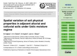
3.2. Models Development and Valuations Remotely sensed data with a significant correlation to EC were considered for developing the regression models. The developed regression models are shown in Figure 2 and their statistical results are summarized in Table 4, showing how well spatial variation in soil salinity can be predicted by applying the different developed regression models. All the developed regression models were highly significant; however, models 1, 2, 3, 4 and 9 were best able to predict soil salinity spatial variation, as they met all the model selection criteria. Among these models, model 4, which combines SI with B3, provided the best fit overall. It had the highest R2, signifying a strongly linear relationship between estimated and predicted EC and indicated that 65% of the variance in the EC values could be explained by this model with relatively low standard errors for its variables at 29.99, 0.52 and 0.26, respectively. Each of these variables had significant p-values, indicating a strong correlation with EC. Figure 2. Scatter plots of predicted vs. measured EC using the developed regression models.
Figure 2. Cont.
Remote Sens. 2014, 6
1144
Table 4. Developed regression models to predict EC based on remotely sensed data. SI, Salinity Index. Model 1
Variable
Regression Coefficient
Standard Error
p-Value
Intercept
−239.49
29.82