Agate Logic Inc. {sayak, alanmi, een, brayton}@eecs.berkeley.edu. {sjang, chaochen}@agatelogic.com. Abstract. Mapping into K-input lookup tables (K-LUTs) is ...
Mapping into LUT Structures Sayak Ray Alan Mishchenko Niklas Een Robert Brayton
Stephen Jang Chao Chen
Department of EECS, University of California, Berkeley
Agate Logic Inc.
{sayak, alanmi, een, brayton}@eecs.berkeley.edu
{sjang, chaochen}@agatelogic.com
Abstract Mapping into K-input lookup tables (K-LUTs) is an important step in synthesis for Field-Programmable Gate Arrays (FPGAs). The traditional FPGA architecture assumes all interconnects between individual LUTs are “routable”. This paper proposes a modified FPGA architecture which allows for direct (non-routable) connections between adjacent LUTs. As a result, delay can be reduced but area may increase. This paper investigates two types of LUT structures and the associated tradeoffs. A new mapping algorithm is developed to handle such structures. Experimental results indicate that even when regular LUT structures are used, area and delay can be improved 7.4% and 11.3%, respectively, compared to the high-effort technology mapping with structural choices. When the dedicated architecture is used, the delay can be improved up to 40% at the cost of some area increase.
1. Introduction LUT-based FPGAs are used already for implementing digital designs in a wide variety of application domains. However, the search for new FPGA architectures and efficient methods of their synthesis remains a continuing area of research. This is motivated by considerations such as reducing delay, area, and power consumption, improving routability and resource utilization, and increasing expressive power of programmable logic. Reducing delay is especially important as it allows high-frequency FPGAs to compete with ASICs. Delay in modern FPGAs is dominated by interconnect. A typical ratio between the intrinsic delay of a LUT and a wire delay is 1:5, because most of the wires are routed through multiple switch-boxes and routing channels. One way to reduce routing delay is to use an FPGA architecture that has direct, or “non-routable”, wires. Such wires can connect two adjacent LUTs in a programmable fabric, possibly at the expense of restricting the fanout count of the LUTs involved. In this paper, we investigate several ways direct wires can be used and experimentally show improvements in delay as a consequence. We call a group of LUTs connected by direct wires, a LUT structure. It can be characterized by the number of interconnected LUTs, their sizes and connectivities. We investigate two single-output LUT structures, “44” and “444”, shown in Figure 1. The connections between the LUTs inside each structure are direct (non-routable), while all other connections are routable. 978-3-9810801-8-6/DATE12/©2012EDAA
4-LUT
4-LUT
4-LUT
4-LUT
4-LUT
Figure 1: The 7-input LUT structure “44” (left) and the 10-input LUT structure “444” (right). In order to investigate the viability of these structures, we had to develop a new mapping algorithm, aimed at efficient implementation into such structures. The contributions of this paper are the following: • Development of an efficient matching algorithm to check if a given Boolean function can be implemented using a given LUT structure. • Modification to the priority-cut-based technology mapper [16] to perform mapping into the LUT structures, as opposed to single LUTs. • Experimental evaluation of the new mapping algorithm applied to regular LUTs as well as the 44 and 444 structures. A promising conclusion is that the algorithm can improve delay and area also for the traditional mapping and substantially improve delay when LUT structures are used. • Statistics on the relative number of k-input Boolean functions, appearing in industrial designs, that can be implemented using the 44 and 444 LUT structures. The paper is organized as follows. Section 2 describes the background and the relevant decomposition theory and Section 3 describes the mapping algorithm. Section 4 reports on some experimental results while Section 5 concludes the paper and outlines future work.
2. Background 2.1 Boolean network A Boolean network (or netlist, or circuit) is a directed acyclic graph (DAG) with nodes corresponding to logic gates and edges corresponding to wires connecting the gates. In this paper, we consider only combinational Boolean networks. A combinational And-Inverter Graph (AIG) is a Boolean network composed of two-input ANDs and inverters. The size (area) of an AIG is the number of its nodes; the depth (delay) is the number of nodes on the longest path from the primary inputs (PIs) to the primary outputs (POs). A cut C of a node n is a set of nodes of the network, called leaves of the cut, such that each path from a
PI to n passes through at least one leaf. Node n is called the root of cut C. For details on cuts and their roles in technology mapping, see [8][16]. We have modified an existing cut-based mapper for mapping into LUTstructures. As usual, a Boolean network is a logical realization of a single or multi-output Boolean function. A single output n Boolean function of n variables is denoted as f : {0,1} •{0,1}, and a multi-output Boolean function is treated as a vector of single-output Boolean functions. We use boldface letters to denote vectors (of variables or functions). A completely-specified Boolean function F essentially depends on a variable if there exists an input combination such that the value of the function changes when the variable is toggled. The support of F is the set of all variables on which function F essentially depends. The supports of two functions are disjoint if they do not contain common variables. A set of functions is disjoint if their supports are pair-wise disjoint. Additional information can be found in the following publications: AIGs [9][4], AIGbased synthesis [14][15], delay optimization and area recovery [6][18].
2.2 Decomposition theory This section reviews the decomposition theory used in Section 4 of this paper. Refer to [12][13][19][20] for details on the traditional decomposition algorithms. For a Boolean function f(X) and a subset of its support, X1, the set of distinct cofactors, q1(X), q2(X), … , qμ(X), of f with respect to (w.r.t.) X1 is derived by substituting all assignments of X1 into f(X) and eliminating duplicated functions. The number of distinct cofactors, μ, is the column multiplicity of f with respect to X1. Given a partition of X into two disjoint subsets, X1 and X2, we say that Ashenhurst-Curtis decomposition of f(X) exists if f(X) can be expressed as f(X) = h( g1(X1), g2(X1), …, gk(X1), X2 ). Subsets X1 and X2 are called the bound set and the free set, respectively. Functions gi(X1), 1 ≤ i ≤ k, are the decomposition functions. Function h(G, X2) is the composition function. The following lemma is useful in subsequent discussions. Lemma 1. [1][7] The decomposition of f(X) with k functions g1(X1), g2(X1), …, gk(X1) exists if and only if ⎡log2μ⎤ ≤ k ≤ n, where μ is the column multiplicity of f with respect to X1, and n = |X1|.
handled using truth tables. For larger functions, BDDs or a mixed AIG/SAT representation is preferable. A special case of checking whether a function can be implemented using a LUT structure, is when the support sizes of the function and the structure are equal. In the case of the LUT structure “XY”, if the support of the function is equal to X + Y – 1, the only case when the decomposition exists, is when the function has a DSD with exactly X variables as a separate block. This check is handled in the pseudo-code below. For example, 5-variable Boolean function F = MUX(c0, d0, MUX(c1, d2, d3)) can be matched with structure “33”, because variables {c1, d2, d3} can be decomposed as a separate block, MUX(c1, d2, d3). On the other hand, this function cannot be matched with structure “24”, because no two variables can be decomposed as a separate block.
3.1 Checking decomposition “XY” Consider decomposition checking for the “XY” structure. The input to the algorithm is an n-input Boolean function and an ordered pair of numbers (X, Y) where 0 ≤ n ≤ 16 and 2 ≤ X,Y ≤ 6. The pseudo-code of the algorithm is shown in Figure 3.1 below. varset performLutMatchingXY( function F, // F is represented using a truth table int X, int Y ) // 2 ≤ X ≤ 6, 2 ≤ Y ≤ 6 { varset V; // a set of Boolean variables int n: // the support size int m; // the column multiplicity // perform support minimization and simple checks n = supportMinimize(F); // removes vacuous variables assert( n ≤ 16 ); if (n ≤ max(X, Y)) return supp(F); if (n > X + Y - 1) return “structure is too small”; // look for the special case decomposition on the output side V = findOutputDecomposition( F, Y-1 ); assert( |V| ≤ Y-1 ); if (n ≤ X + |V|) return supp(F) - V; // look for a good bound-set in the direct variable order (V, m) = findGoodBoundSet( F, X ); assert( |V| ≤ X ); if (m == 2) if (n ≤ |V| + Y – 1) return V; if (3 ≤ m ≤ 4 && n ≤ |V| + Y – 2) if ( checkSpecialNonDisjoint(F, V) ) return V;
3. Algorithm We use a notation for the LUT structures, e.g. “XY” or “XYZ”, where the last character represents the root node and the first one or two characters represent the nodes feeding into it. For example, “345” represents a structure where a node of size 3 and a node of size 4 feed directly into a node of size 5. This section describes an efficient algorithm to determine whether a Boolean function can be implemented in “XY” or “XYZ”, 2 ≤ k ≤ 6, k ∈ {X, Y, Z}. The node size does not exceed 6 because most FPGAs are based on LUTs of 6 inputs or less. The support size of a function is limited to 16, because the truth table representation works well for such functions. In general, if runtime is not an issue, functions up to 20 inputs can be
// look for a good bound-set in the reverse variable order reverseVariableOrder( F ); (V, m) = findGoodBoundSet( F, X ); assert( |V| ≤ X ); if (m == 2) if (n ≤ |V| + Y – 1) return V; if (3 ≤ m ≤ 4 && n ≤ |V| + Y – 2) if ( checkSpecialNonDisjoint(F, V) ) return V; return “decomposition does not exist”; }
Figure 3.1. LUT matching for two-node structure “XY”. The LUT matching uses procedure supportMinimize(), which removes vacuous variables and returns the new support size. For example, assuming that the variable order is (a,b,c,d), function F = acd has the vacuous variable b.
Support minimization removes variable b from the support, resulting in function G = abc, whose support size is 3. If n • max(X,Y), the function can be packed into one node, while the other node can be treated as a buffer. If n > X + Y – 1, decomposition does not exist because the LUT structure is too small. Procedure findOutputDecomposition() checks for a special case of decomposition, F = x ⊗ G, where ⊗ is a two variable Boolean function, x is a support variable, and G is a remainder function. For this, single-variable cofactors of F are checked and the following three special cases are considered: a constant-0 cofactor (AND-decomposition), a constant-1 cofactor (OR-decomposition), and two cofactors that are complements of each other (XOR-decomposition). Note that a pair of cofactors cannot be equal, because after support minimization, F depends on all its variables. If the simple decomposition exists for one variable x, the check is iteratively applied to the remainder function G and its remainders, if any, until the number of decomposed variables is equal to Y-1. The decomposed variables are returned by the procedure findOutputDecomposition(). If the variable set returned is not enough to decompose the function, procedure findGoodBoundSet(), attempts are made to find a good bound set. This procedure tries to reorder variables in the truth table while minimizing the column multiplicity with respect to the topmost X variables. Reordering of variables in a truth table is similar to that in for BDDs, but typically is faster because a procedure has been developed, which swaps variables i and j directly, without going through a sequence of adjacent variable swaps, known as variable sifting for BDDs. The best column multiplicity and variable set are returned. If the column multiplicity is 2 and the number of variables in the set is sufficiently large (n ≤ |V| + Y – 1), the variable set is returned. Otherwise, a non-disjoint decomposition with one shared variable is attempted [12]. If such decomposition exists, the variable set is returned. If decomposition is not found, the variable order is reversed and findGoodBoundSet() is called again. Reversing the variable order is a heuristic used for hard-tomatch functions, even though it does not guarantee that the match is always found if it exists. The reversing of the variable order can be done efficiently on a truth table. An additional optimization omitted in the pseudo-code of Figure 3.1, is that of caching previously computed results. Thus, when decomposition checking is applied repeatedly to the same function, it is retrieved from the cache, instead of running the check from scratch.
3.2 Checking decomposition “XYZ” The input to the algorithm is an ordered set of integers (X, Y, Z) and a n-input Boolean function F, 0 ≤ n ≤ X + Y + Z - 2, where 2 ≤ X,Y,Z ≤ 6 and 0 ≤ n ≤ 16. The decomposition check in this case is implemented as two checks: checking F for decomposition using “XW”, where W = Y + Z – 2. If it exists, the remainder function G is checked for decomposition using structure “YZ”. To ensure that the resulting structure has blocks “X” and “Y” feeding directly into block “Z”, instead of block “X” feeding into block “Y” and block “Y” feeding into block “Z”, the algorithm in Figure 3.1 is modified slightly. When
the feasibility checks are performed, the output variable of the first block “X” is not included into the variable sets returned by the checking procedures.
3.3 Modifying the technology mapper The priority-cut-based technology mapper [16] needed to map into the “XY” and “XYZ” LUT structures allows the user to define custom cost functions for evaluating cuts during mapping. In the case of mapping into the “44” (”444”) structures, the mapper performs enumeration of 7-input (10-input) cuts, computes their cut functions as truth tables, and checks the decomposition for each cut function. If the function is not decomposable, the cut is skipped. If it is decomposable, the area and delay of the resulting cut are defined using the number of inputs of the function, as specified in the given LUT library. A LUT library lists delay and area of the LUT of each size. Examples of LUT libraries are given in Section 5. The mapper minimizes the delay of the mapping, followed by several rounds of heuristic area recovery. When the user-specified cost functions are employed, as described above, all the cuts used in the mapping have Boolean functions decomposable into the “XY” or “XYZ” LUT structures.
4. Experimental results The proposed algorithm is implemented in ABC [2][4] as part of the priority-cut-based technology mapper [16] (command if). The following are the relevant switches that have been added to the technology mapper: • -S 44 enables mapping into “44” structure, • -S 444 enables mapping into “444” structure, • -K specifies the cuts size. Experiments were performed using a suite of public benchmarks and a suite of industrial benchmarks.
4.1 Improvements to traditional mapping In the first experiment, reported in Table 4.2, the target structure is the traditional 4-LUT FPGA. In this case, when switch “-S” is used, the delay/area of the LUT structure “44” (“444”) are the same as the area/delay of two (three) 4-LUTs. The following runs are performed and reported in the columns of Table 4.2. The notation (cmd1; cmd2)n means that cmd1 followed by cmd2 was iterated n times. • Baseline: This runs if with LUT Library L1 shown in Table 4.1. Note that this library specifies unit-delay and unit-area for each LUT up to size 4. • Mapping with structural choices (MSC): This runs (dch; if)4 using the Library L1. • 44: This runs (dch; if –S 44)4 with Library L2. This library specifies delay/area equal to 1 for each LUT up to size 4, and equal to 2 for larger LUTs. • 444: This runs (dch; if -S 444)4 using Library L4. This library specifies delay/area equal to 1 for each LUT up to size 4, and delay/area equal to 2 or 3 for larger cuts. • Best 444: This runs (dch; if -S 444)4 using Library L5. This library estimates the quality of mapping into the LUT structure “444”. For each cut size, the library contains the approximate number of LUTs needed to implement it, assuming that 50% of 7-
input functions are mapped into two 4-LUTs and 50% are mapped into three 4-LUTs. Table 4.2 shows that, when the proposed algorithm is used, both area and delay are improved, compared to mapping with structural choices (MSC). For example, when mapping is performed using 7-input cuts matched with the “44” LUT structures composed of two 4-LUTs, the area and delay are improved by 4.6% and 6.1%, respectively. When mapping using 10-input cuts matched with the “444” LUT structures composed on three 4-LUTs, the area and delay are improved by 7.4% and 11.3%, respectively.
4.2 Delay-optimization using LUT structures In this experiment, reported in Table 4.3 and Table 4.4, we assume that FPGA hardware allows for efficient realization of the “44” and “444” structures with direct (non-routable) connections between the adjacent LUTs. The runs performed are the same as in the previous experiment (Section 4.1), except that the delay of the direct connection is assumed to be 1.2 instead of 2. The updated LUT libraries are listed below: 44 (Library L3), 444 (Library L6), Best 444 (Library L7). The results of this experiment show that the delay can be substantially reduced at the cost of some increase in area, compared to mapping with structural choices (MSC). Consider Table 4.3 as an example. When mapping is performed using 7-input cuts matched with the “44” LUT structures, the delay is reduced by 28.2% while the area is increased by 5.1%. When mapping is performed using the “444” LUT structures, the delay is reduced by 43.2% while the area is increased by 14.1%. The area increase may be prohibitive and will be addressed as part of future work.
4.3 The ratios of realizable functions In a separate experiment not shown in the tables, we evaluated the relative number of 7-input (10-input) functions appearing in the circuits that can be matched with the “44” (“444”) LUT structures. The results differ for the industrial designs and for the public benchmarks listed in Tables 4.2 and 4.3. For the industrial designs, 97% (70%) of 7-input (10-input) functions can be matched with the “44” (“444”) LUT structure. For the public benchmarks, the numbers are 99% and 84%, respectively. It is surprising that such a high percentage of cuts have Boolean functions that can be matched with the LUT structures.
When the algorithm is used to map into this architecture, the delay improvement can be up to 40% at the cost of some area increase. Future work will explore whether the delay reductions reported in this paper translate into improved maximum clock frequency (Fmax) after place-and-route.
6. Acknowledgements This work has been supported in part by contacts from SRC (1875.001), NSA, and industrial sponsors: Actel, Altera, Atrenta, Cadence, Calypto, IBM, Intel, Jasper, Magma, Oasys, Real Intent, Synopsys, Tabula, and Verific.
7. REFERENCES [1]
[2] [3] [4] [5] [6] [7] [8] [9] [10] [11] [12] [13] [14] [15] [16]
5. Conclusions This paper proposes an improvement to technology mapping for FPGAs. The main idea is to reduce structural bias by mapping into LUT structures composed of two or three 4-LUTs. The experimental results indicate that the new algorithm can improve both area and delay of the traditional technology mapping. Additionally, an FPGA architecture allowing for direct connections between pairs of adjacent LUTs is evaluated.
[17] [18] [19] [20]
R. L. Ashenhurst, “The decomposition of switching functions”, Proc. Intl Symposium on the Theory of Switching, Part I (Annals of the Computation Laboratory of Harvard University, Vol. XXIX), Harvard University Press, Cambridge, 1959, pp. 75-116. Berkeley Logic Synthesis and Verification Group. ABC: A System for Sequential Synthesis and Verification. http://wwwcad.eecs.berkeley.edu/~alanmi/abc V. Bertacco and M. Damiani. "The disjunctive decomposition of logic functions". Proc. ICCAD '97, pp. 78-82. R. Brayton and A. Mishchenko, "ABC: An academic industrialstrength verification tool", Proc. CAV'10, LNCS 6174, pp. 24-40. S. Chatterjee, A. Mishchenko, R. Brayton, X. Wang, and T. Kam, “Reducing structural bias in technology mapping”, ICCAD '05. J. Cong and Y. Ding, “FlowMap: An optimal technology mapping algorithm for delay optimization in lookup-table based FPGA designs”, IEEE Trans. CAD, vol. 13(1), Jan. 1994, pp. 1-12. A. Curtis. New Approach to the Design of Switching Circuits. Van Nostrand, Princeton, NJ, 1962. R. J. Francis, J. Rose, and K. Chung, ”Chortle: A technology mapping program for lookup table-based field programmable gate arrays”, Proc. DAC ’90, pp. 613-619. A. Kuehlmann, V. Paruthi, F. Krohm, and M. K. Ganai, “Robust boolean reasoning for equivalence checking and functional property verification”, IEEE TCAD, Vol. 21(12), Dec. 2002, pp. 1377-1394. E. Lehman, Y. Watanabe, J. Grodstein, and H. Harkness, “Logic decomposition during technology mapping,” IEEE Trans. CAD, Vol. 16(8), Aug. 1997, pp. 813-833. A. Mishchenko, B. Steinbach, and M. A. Perkowski, "An algorithm for bi-decomposition of logic functions", Proc. DAC '01, 103-108. A. Mishchenko and T. Sasao, "Encoding of Boolean functions and its application to LUT cascade synthesis", Proc. IWLS '02, 115-120. A. Mishchenko, X. Wang, and T. Kam, "A new enhanced constructive decomposition and mapping algorithm", Proc. DAC '03, pp. 143-148. A. Mishchenko, S. Chatterjee, and R. Brayton, "DAG-aware AIG rewriting: A fresh look at combinational logic synthesis", Proc. DAC '06, pp. 532-536. A. Mishchenko and R. K. Brayton, "Scalable logic synthesis using a simple circuit structure", Proc. IWLS '06, pp. 15-22. A. Mishchenko, S. Cho, S. Chatterjee, R. Brayton, “Combinational and sequential mapping with priority cuts”, Proc. ICCAD ’07, pp. 354-361. A. Mishchenko, R. Brayton, and S. Jang, "Global delay optimization using structural choices", Proc. FPGA'10, pp. 181-184. P. Pan and C.-C. Lin, “A new retiming-based technology mapping algorithm for LUT-based FPGAs,” Proc. FPGA’98, pp. 35-42. J.-H. R. Jiang, J.-Y. Jou, and J.-D. Huang. “Compatible class encoding in hyper-function decomposition for FPGA synthesis," Proc. DAC’98, pp. 712-717. W.-Z. Shen, J.-D. Huang, and S.-M. Chao, “Lambda set selection in Roth-Karp decomposition for LUT-based FPGA technology mapping”, Proc. DAC’95, pp. 65–69.
Table 4.1. LUT libraries used in the experimental results.
1-4 5-6
1 2
1 2
7 8-10
2.5 3
2 2
1-4 5-10
1 3
1 1.2
delay
1 2
Library L7 area
1 3
#k
delay
1-4 5-10
#k
Library L6 area
1 1.2
delay
1 2
Library L5 area
1-4 5-7
delay
1 2
#k
area
1 2
#k
Library L4
delay
1-4 5-7
Library L3 area
1
#k
delay
1
Library L2 area
1-4
delay
#k
area
Library L1
1-4 5-6
1 2
1 1.2
7 8-10
2.5 3
1.2 1.2
#k
Table 4.2. Improvements to the traditional FPGA mapping. Profile Designs
PI
PO
LUTs FF
Basic
MSC
44
Levels 444
Best
Basic
MSC
44
Runtime (secs) 444
Best
MSC
44
44
Best
alu4
14
8
0
705
688
635
584
567
9
7
7
7
7
2
5
14
12
apex2
39
3
0
961
799
691
611
554.5
9
8
7
7
7
4
7
15
14
b14
32
54
245
2295
1750
1678
1647
1671.5
22
20
19
17
16
7
38
78
55
b15
36
70
449
3293
3022
2910
3009
3067.5
23
22
22
19
18
19
58
98
78
b17
37
97
1415
10392
9271
8957
8919
9029.5
34
31
30
26
26
62
162
276
277
b20
32
22
490
4510
3523
3361
3386
3329
23
22
22
20
20
16
84
169
130
b21
32
22
490
4758
3512
3359
3304
3338
23
22
22
21
21
17
79
131
128
b22
32
22
735
6727
5255
4971
4953
4997
24
22
22
21
21
25
97
208
207
clma
383
82
33
3872
3766
3358
2814
2460
17
13
12
11
11
27
62
91
57
des
256
245
0
1242
1213
1172
1077
1053.5
8
6
6
6
6
3
16
37
38
19
2
194
377
428
415
414
417.5
11
8
8
8
8
1
2
3
4
8
63
0
514
463
443
433
432
12
6
5
5
5
1
5
15
14 80
elliptic ex5p frisc
4
116
886
2242
2220
2108
2223
2239.5
21
19
18
14
14
11
30
76
i10
257
224
0
739
733
747
766
752
19
14
12
11
12
2
8
23
24
pdc
16
40
0
2232
2039
1923
1951
1921
13
8
8
8
8
20
45
107
84
s38584
13
278
1452
4234
3942
3805
3668
3779
11
8
8
7
7
11
35
32
35
s5378
36
49
161
467
445
446
436
436.5
7
6
5
5
5
1
3
7
6
seq
41
35
0
979
908
830
734
724.5
8
6
6
6
6
4
9
23
20
spla
16
46
0
2168
1900
1858
1838
1850
13
9
8
8
8
17
42
96
70
tseng
52
122
385
Geomean Ratio1 Ratio2 Ratio3 Ratio4
837
740
744
738
759.5
13
13
10
10
9
2
6
14
15
1772 1
1598 0.902 1
1524 0.860 0.954 1
1479 0.835 0.926 0.970 1
1464 0.826 0.916 0.961 0.990
14.51 1
11.67 0.804 1
10.96 0.755 0.939 1
10.35 0.713 0.887 0.944 1
10.28 0.708 0.881 0.938 0.993
6.59 1
20.68 3.138 1
42.67 6.474 2.063 1
38.78 5.885 1.875 0.909
Table 4.3. Delay-optimization using dedicated FPGA architecture with direct connections between adjacent LUTs. Profile Designs
PI
PO
LUTs FF
Base
MSC
44
Levels 444
Best
Base
MSC
44
Runtime (secs) 444
Best
MSC 44
444
Best
alu4
14
8
0
705
688
664
685
634
9
7
5.6
4.6
4.6
2
5
12
11
apex2
39
3
0
961
799
822
829
774.5
9
8
6
4.8
4.8
4
7
16
14
b14
32
54
245
2295
1750
1806
2067
2127
22
20
14
10.6
10.6
8
33
108
70
b15
36
70
449
3293
3022
3274
3656
3900.5
23
22
15.4
11.8
10.8
19
55
81
86
b17
37
97
1415
10392
9271
9596
10182
10446
34
31
20.8
15.4
14.4
63
154
276
309
b20
32
22
490
4510
3523
3830
4552
4592
23
22
14.2
10.8
10.8
16
67
147
134
b21
32
22
490
4758
3512
3867
4394
4413
23
22
14.2
10.8
10.8
17
78
184
134
b22
32
22
735
6727
5255
5749
6801
6770.5
24
22
15.4
10.8
10.8
24
96
199
212
clma
383
82
33
3872
3766
3771
3528
3710.5
17
13
9.4
8
7
28
53
131
53
des
256
245
0
1242
1213
1246
1047
1267.5
8
6
4.6
4.4
3.6
3
16
42
43
19
2
194
377
428
456
476
466
11
8
6.6
5.8
5.6
1
1
4
3
elliptic ex5p
8
63
0
514
463
498
527
483.5
12
6
4.6
3.4
3.4
1
6
10
9
frisc
4
116
886
2242
2220
2442
2618
2678.5
21
19
10.6
8.2
8.2
10
29
72
76
i10
257
224
0
739
733
772
882
884
19
14
9.4
7.2
7.2
2
8
24
25
pdc
16
40
0
2232
2039
2604
3043
2855
13
8
6.8
5.8
5.8
21
41
111
62
s38584
13
278
1452
4234
3942
3448
3950
3881
11
8
6.8
4.6
4.8
11
32
63
64
s5378
36
49
161
467
445
390
476
497.5
7
6
4.4
3.6
3.4
1
4
6
7
seq
41
35
0
979
908
927
887
826
8
6
4.8
4.6
4.6
4
8
22
22
spla
16
46
0
2168
1900
2315
2769
2691
13
9
7
5.8
5.8
18
45
49
51
tseng
52
122
385
837
740
797
931
826.5
13
13
7
4.8
5.8
1
6
14
9
Geomean
1772
1598
1679
1824
1814
14.51
11.67
8.38
6.63
6.52
6.42
19.54
43.55
37.82
1
0.902
0.948
1.029
1.024
1
0.804
0.578
0.457
0.449
1
3.045
6.787
5.894
1
1.051
1.141
1.135
1
0.718
0.568
0.558
1
2.229
1.936
1
1.086
1.080
1
0.791
0.777
1
0.868
1
0.994
1
0.983
Ratio1 Ratio2 Ratio3 Ratio4
Table 4.4. Delay-optimization using dedicated FPGA architecture with direct connections between adjacent LUTs for industrial designs. LUT Designs D1 D2 D3 D4 D5 D6 D7 D8 D9 D10 D11 D12 D13 D14 D15 Geomean Ratio1 Ratio2 Ratio3 Ratio4
Base 1437 1455 1565 1831 2901 2908 3235 3605 4421 4540 5743 6063 6238 10248 27896 3900 1
MSC 1344 1405 1540 1734 2787 2746 3093 3249 3851 4323 4415 6248 6236 9227 23793 3624 0.929 1
44 1397 1540 1667 1713 2715 2776 3099 3412 3417 4337 4899 5096 6994 9171 23395 3650 0.936 1.007 1
Levels 444 1320 1411 2187 1724 2742 2888 2984 3300 3532 4272 5545 6759 7619 8962 23833 3803 0.975 1.050 1.042 1
Best 1363.5 1410.5 1952.5 1726.5 2753.5 2882.5 3012.0 3840.0 3547.0 4343.5 5365.5 6498.5 8124.0 8657.0 24276.0 3824 0.980 1.055 1.048 1.005
Base 15.0 8.0 14.0 11.0 15.9 10.0 14.9 20.0 7.0 19.0 15.0 12.0 9.0 13.9 17.0 12.88 1
MSC 13.0 8.0 13.0 8.3 14.0 10.0 13.4 15.0 7.0 16.9 15.0 10.0 9.0 13.5 17.0 11.77 0.914 1
44 10.2 5.6 8.0 6.1 11.4 7.0 11.6 11.6 5.6 10.6 12.6 8.2 7.2 11.8 13.0 8.99 0.698 0.764 1
444 9.9 4.8 4.8 5.9 11.2 5.8 11.1 11.8 6.0 11.8 10.6 7.0 7.0 11.2 11.4 8.23 0.639 0.699 0.915 1
Best 9.5 4.6 4.6 6.0 11.3 5.8 10.8 10.8 6.0 11.3 10.8 7.0 7.0 11.5 11.0 8.09 0.628 0.687 0.900 0.983