Massively Parallel Large Scale Stokes Flow Simulation - JuSER

Massively Parallel Large Scale Stokes Flow Simulation B. Gmeiner, M. Huber, L. John, U. Rude, C. Waluga, ¨ B. Wohlmuth

published in

NIC Symposium 2016 K. Binder, M. Muller, M. Kremer, A. Schnurpfeil (Editors) ¨ Forschungszentrum Julich GmbH, ¨ John von Neumann Institute for Computing (NIC), Schriften des Forschungszentrums Julich, NIC Series, Vol. 48, ¨ ISBN 978-3-95806-109-5, pp. 333. http://hdl.handle.net/2128/9842

c 2016 by Forschungszentrum Julich

¨ Permission to make digital or hard copies of portions of this work for personal or classroom use is granted provided that the copies are not made or distributed for profit or commercial advantage and that copies bear this notice and the full citation on the first page. To copy otherwise requires prior specific permission by the publisher mentioned above.

Massively Parallel Large Scale Stokes Flow Simulation ¨ 1, Bj¨orn Gmeiner1 , Markus Huber2 , Lorenz John2 , Ulrich Rude 2 2 Christian Waluga , and Barbara Wohlmuth 1

2

Institute of System Simulation, University Erlangen-Nuremberg, 91058 Erlangen, Germany E-mail: {bjoern.gmeiner,ulrich.ruede}@fau.de Department of Mathematics, Technische Universit¨at M¨unchen, 85748 Garching, Germany E-mail: {huber,john,wohlmuth}@ma.tum.de In many applications, physical models consisting of a Stokes-type equation that is coupled to a convection-dominated transport equation play an important role, e.g., in mantle-convection or ice-sheet dynamics. In the iterative treatment of such problems the computational cost is usually dominated by the solution procedure for the Stokes part. Hence, we focus on massively scalable and fast multigrid solvers for the arising saddle point problem. To gain deeper insight into the performance characteristics, we evaluate the multigrid efficiency systematically and address the methodology of algorithmic resilience. Three methods based on the HHG software framework will be presented and are shown to solve FE systems with half a billion unknowns even on standard workstations. On petascale systems they furthermore exhibit excellent scalability. This together with the optimised performance on each node leads to superior supercomputing efficiency. Indefinite systems with up to ten trillion (1013 ) unknowns can be solved in less than 13 minutes compute time.

1

Introduction

Thanks to the continuous improvements made in parallel computing technology, current leading-edge supercomputers can provide up to several petaflop/s of performance provided that suitable algorithms and implementations are designed. While this enables the development of increasingly complex computational models with unprecedented resolution, it also requires a novel co-design process that aims at maximal performance at all stages of developing a simulator. This includes the appropriate choice of mathematical models, discretisations, and algorithms, as well as the matter of software implementation, which all – in their interplay – must be carefully analysed, adapted, and possibly revised to avoid unnecessary inefficiencies in data volume, data traffic, and arithmetic cost. To achieve several levels of parallelism with hundreds of thousands of threads all components must be specifically designed for avoiding synchronisation and communication where possible. This often requires the use of complex hybrid programming models. In this work, we use the hierarchical hybrid grids framework (HHG)1, 2 that realises a compromise between structured and unstructured grids. It exploits the flexibility of finite elements and capitalises on the algorithmic efficiency of geometric multigrid methods. The HHG package was initially designed with scalar elliptic equations in mind, see Refs. 1, 2. In Refs. 5, 6 an extension to Stokes systems using a pressure-correction scheme was presented and in Ref. 12 we discuss the conservative coupling to transport equations. For the extension to other types of scalable multigrid-based Stokes solvers, see Ref. 10. In the context of multigrid methods, the execution of a parallel smoothing step for the multigrid algorithm consumes a major part of the total computational cost. The performance of such

333

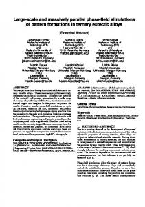
algorithms can be substantially improved, e.g. by using suitable discretisations that permit a memory-efficient, matrix-free implementation. Our application problem is motivated by fundamental geophysical questions revolving around the physics of the Earth’s mantle, which extends from some tens of kilometres below the surface down to the core-mantle-boundary at about 2 900 km depth. In this region, convection patterns of solid material evolve on large time- and length-scales; e.g., Fig. 1 shows the rise of a typical plume formation, displaying the characteristic “mushroom” shape of the iso-temperature surfaces.

Figure 1. Scaled temperature distribution for a coupled convection simulation. The convective part of the energy balance equation is determined by the velocity solution of a Stokes system.

While the general structure of convection within the mantle is relatively well understood, some important details remain open, including the potential thermo-chemical nature of the convection currents (which are essentially a statement on the buoyancy forces) appropriate rheological parameters and the importance of lateral viscosity variation11 . Due to the extreme conditions deep inside the Earth and the large time scales involved, answering these questions is mostly outside the scope of laboratory experiments. Thus, further progress in mantle convection research relies on extracting meaningful answers from the geologic record through a careful assimilation of observations into models by means of fluid dynamics inverse simulations3 . There are three aspects making the inversion feasible: the strongly advective nature of the heat transport, the availability of terminal conditions from seismic tomography, providing current temperatures and densities inside the mantle, and the availability of boundary conditions, i.e. surface velocity fields for the past 130 million years, from paleomagnetic reconstructions.

2

Simulation Models

A popular model for mantle convection considers the conservation of mass, momentum and energy in the following form:

334

− div σ = ρg

∂t ρ + div(ρu) = 0

∂t (ρe) + div(ρeu) = − div q + H + σ : ε˙

(1a) (1b) (1c)

Here, σ represents the stress tensor while ε˙ = 21 (∇u + ∇u> ) denotes the rate of strain tensor that is defined as the symmetric part of the gradient of the velocity field u. The vector g denotes the gravitational acceleration acting in vertical/radial direction. We further denote the internal energy density by e, the heat flux per unit area by q, and the volumetric radiogenic heat production rate by H. The density ρ = ρ(p, T ) is related to the pressure p and the temperature T through an equation of state that is investigated in the field of mineralogy and usually represented via lookups or analytical expressions. Finally, the stress tensor σ is defined as σ = 2µ(ε˙ −

1 3

tr ε˙ · I) − pI,

(2)

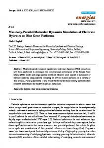
where µ denotes the dynamic viscosity. As mentioned before, the rheology of the mantle is not yet well understood4 , and there are different models for the viscosity. As the focus of this present study is on parallel scalability and efficiency, we only consider numerical examples for a simplified model of mantle convection in the following. Firstly, we employ the Boussinesq-approximation, i.e., we treat the flow as incompressible everywhere apart from the buoyancy term ρg. The mass balance (Eq. 1b) then simplifies to the incompressibility constraint div u = 0. It is well-known that for long term dynamic simulations of coupled problems, local mass conservation is a crucial ingredient. Although we are using stabilised P1 conforming finite element spaces for the velocity and the pressure space, our simulation results do not suffer from the lack of mass conservation. A local post-process7, 12 guarantees that the velocity flux entering the energy balance equation is locally conservative, and thus no spurious source or sink terms occur. The picture on the right of Fig. 2 shows the vorticity field produced by the modified approach which is in excellent agreement with the reference solution while the one on the left exhibits a physically incorrect structure.

Figure 2. Uncorrected (left) vs. corrected (right) coupling approach: Vorticity contour surfaces for an isoviscous Boussinesq flow with free-slip conditions and a Rayleigh-number of Ra = 7.7 · 104 .

335

If we additionally assume a constant viscosity, the model can be even further simplified and instead of the symmetric strain operator, we can use the gradient operator in the momentum equation (Eq. 1a) which has the advantage that the different velocity components decouple, and the associated stencils are smaller. By doing so, roughly a factor of two in the time-to-solution can be saved.

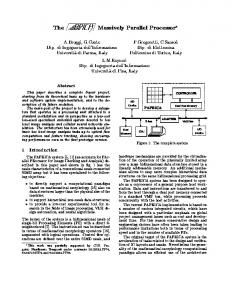
Figure 3. Domain with ns = 305 equally sized, randomly placed spheres and velocity streamlines.

It should be mentioned that our HHG solver is not tailored towards the spherical shell geometry. For instance, in Fig. 3 we present the velocity streamlines of the flow through a cylindrical channel filled with randomly place spheres on which we impose no-slip boundary conditions. In Fig. 4, we illustrate the effect of different radii. Setups of this type are of relevance for instance when studying infiltration processes.

Figure 4. Domain with ns = 231 randomly placed spheres with three different radii and velocity streamlines.

3

Parallel Multigrid Performance

For the solution of the simplified mantle-convection problem on the spherical shell domain we usually consider an iterative coupling, where we solve the mass-momentum system and

336

the energy equation separately. Since the first part constitutes the most challenging part, we shall in the following employ and compare different solver strategies. Given a fast solver for a scalar positive definite system, the most natural approach to extend the existing framework to the indefinite Stokes system is to consider the Schur complement for the pressure. After formally performing an elimination of the velocity, the discrete problem for the pressure reads as (3)

Sp = r.

Here S stands for the pressure Schur complement which is defined by S = BA−1 B> +C, where A stands for the discrete velocity operator in the momentum balance equation, B denotes the discrete divergence operator, and C is the matrix resulting from the stabilisation term that suppresses spurious pressure modes resulting from the equal-order approximation (we use a P1 − P1 approximation below). The right-hand side is given by r. In our numerical experiments, we solve Eq. 3 by a preconditioned conjugate gradient method, where we choose a lumped mass matrix preconditioner that is known to be spectrally equivalent to S; see e.g. Ref. 8. This simple preconditioning reduces the effects of varying element sizes and shapes and can be extended to account for non-isoviscous flow. Since the direct assembly of the dense matrix S cannot be performed efficiently, it is applied indirectly by replacing each multiplication of the discrete inverse A−1 by a few cycles of a parallel geometric multigrid algorithm. In addition to the previously described strategy we consider two competing approaches that deal directly with the indefinite nature of the system. The first one is a preconditioned Krylov space method and the second one a multigrid method applied directly to the saddle-point system. This method employs an Uzawa type smoother10 . To obtain a better understanding of the different solvers, we first run the solvers on a conventional, low cost workstation for the serial case with a single Intel Xeon CPU E2-1226 v3, 3.30 GHz and 32 GB shared memory.

L 2 3 4 5 6 7

DoFs 1.4 · 104 1.2 · 105 1.0 · 106 8.2 · 106 6.6 · 107 5.3 · 108

SCG iter time 26 0.11 28 0.56 28 3.33 28 24.28 31 205.84 out of memory

MINRES iter time 108 0.23 83 0.78 73 3.99 70 26.53 67 189.27 out of memory

MG Uzawa iter time 9 0.08 8 0.29 8 1.79 8 12.70 8 95.85 8 730.77

Table 1. Iteration numbers and time-to-solution (in sec.) on standard workstation for a constant viscosity.

Roughly speaking, the three approaches based on HHG outperform most competing methods significantly and reach on a workstation the performance when less efficient methods may already require a supercomputer. Beyond this, the multigrid method for the indefinite system with a suitable Uzawa type smoother (MG-Uzawa) outperforms the two alternative approaches with respect to memory and time-to-solution. Tab. 1 shows in detail that with our co-design it is already possible to solve indefinite systems with half a billion unknowns in a few minutes on a standard low cost machine. To further investigate the

337

characteristics of the different approaches, we identify the required operator applications for all solvers in the same setting. To enable a fair comparison the stopping criteria for all solvers are chosen in exactly the same way. In our results, which we depict in Fig. 5, it can be observed that the Uzawa multigrid method for the indefinite system requires considerably fewer operator evaluations of the operator A and consequently requires a shorter runtime. This effect is expected to become even more significant when considering more complex models, e.g., with varying viscosities.

# operator evaluations

500

A

B

C

M

400 300 200 100 0 SCG

MINRES

MG Uzawa

Figure 5. Number of different operator evaluations for the three considered solvers.

Let us next restrict ourselves to the Uzawa multigrid method (MG-Uzawa) and demonstrate some weak scaling results obtained on the JUQUEEN supercomputer (J¨ulich Supercomputing Centre, Germany), currently listed in the top 10 of the TOP500 lista . In our numerical results that are presented in Tab. 2, we observe robustness with respect to the problem size and excellent scalability. Additionally to the time-to-solution (time) we present the time without coarse grid (time w.c.g.) and the total amount in % which is needed to solve the coarse grid problems. To approximate the coarse grid problem, we apply a preconditioned Krylov subspace solver. It can be observed that even for the largest example computation, the latter fraction is smaller than one-eighth of the total run-time. The largest problem exceeds 1013 unknowns. Nodes

Threads

5 40 320 2 560 20 480

80 640 5 120 40 960 327 680

DoFs 9

2.7 · 10 2.1 · 1010 1.2 · 1011 1.7 · 1012 1.1 · 1013

iter 10 10 10 9 9

time

time w.c.g.

time c.g. in %

685.88 703.69 741.86 720.24 776.09

678.77 686.24 709.88 671.63 681.91

1.04 2.48 4.31 6.75 12.14

Table 2. Weak scaling results with and without coarse grid for the spherical shell geometry.

a http://top500.org

338

4

Fault Tolerant Algorithms

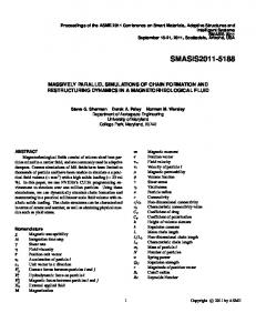
In the future era of exa-scale computing systems, highly scalable implementations will execute up to billions of parallel threads on millions of compute nodes. In this scenario, fault tolerance will become a necessary property of hardware, software and algorithms. Nevertheless, nowadays commonly used redundancy approaches, e.g., check-pointing, will be too costly, due to the high memory and energy consumption. An alternative and less consuming approach is to incorporate resilient strategies directly into the multigrid solver. In Ref. 9, we introduce a methodology and data-structure to efficiently recover lost data due to a processor crash (hard fault) when solving elliptic PDEs with multigrid algorithms. We consider a fault model where a processor stores the mesh data of a subdomain including all its refined levels in the multigrid hierarchy. Therefore, in case of a processor failure, we assume that all data is lost in the faulty domain ΩF ⊂ Ω. We further assume that the healthy domain ΩH ⊂ Ω is unaffected by the fault, and data in this domain remains available. The nodes associated with the interface Γ := ∂ΩF ∩∂ΩH between the faulty and healthy domain are used to communicate between neighbouring processors by introducing ghost copies that redundantly exist on different processors. Therefore, a complete recovery of these nodes is possible without additional storage. To recover the nodal values (uF , pF ) in ΩF which are lost during a fault, we propose to solve a local Stokes (subproblem in ΩF ) with Dirichlet boundary conditions on Γ for velocity and pressure, respectively. To guarantee that the local system is uniformly well-posed, we formally include a compatibility condition obtained from the normal components of the velocity. If the local solution in ΩF is computed while the global process is halted, then this procedure yields a local recovery strategy. In Ref. 9 this local strategy is extended to become a global recovery strategy. To this end, the solution algorithm proceeds asynchronously in the faulty and the healthy domain such that no process remains idle. Temporarily, the two subdomains are decoupled at the interface Γ, and the recovery process in the faulty domain is accelerated by delegating more compute resources to it. This acceleration is termed the superman strategy. Once the recovery has proceeded far enough and has caught up with the regular solution process, both subdomains are re-coupled and the regular global iteration is resumed. These approaches result in a time- and energyefficient recovery. In Fig. 6 (left), we consider a test scenario in Ω = (0, 1)3 in which we continuously apply multigrid V(3,3)-cycles of the Uzawa multigrid method introduced in Sec. 3. In total 23 iterations are needed to reach the round-off limit of 10−15 . During the iteration, a fault is provoked after 5 iterations affecting 2.1% of the pressure and velocity unknowns. As approximate subdomain solvers we compare the fine grid Uzawa-smoother, the minimal residual method, the block-diagonal preconditioned MINRES (PMINRES) method and V, F, W-cycles in the variable smoothing variant from Sec. 3. For the blockpreconditioner in case of PMINRES a standard V-cycle and a lumped mass-matrix M are used. Fig. 6 (left) displays also the cases in which no fault appears (fault-free) and when no recovery is performed after the fault. After the fault, we observe that the residual jumps up and when no recovery is performed, the iteration must start almost from the beginning. A higher pre-asymptotic convergence rate after the fault helps to catch up, so that only four additional iterations are required. This delay can be further reduced by a local recovery computation, but only local multigrid cycles are found to be efficient recovery methods.

339

FAULT & RECOVERY

100

−4

Residual

10

10−8

10−12

10−16

0

5

Fault-Free Fault 4×Vcycle 4×Wcycle 4×Fcycle 50×Smooth

Size 7693 1 2813 2 3053 4 3533

50×MINRES 20×PMINRES

5

10

15

Iterations

20

DN Strategy ηsuper = 4 nH = 0 2 3 4 19.21 0.05 -0.38 4.22 21.27 -0.15 -0.68 3.95 18.50 -0.33 -0.87 3.76 19.74 2.58 4.61 9.24

25

Figure 6. Laplace problem: left: Convergence of the relative residual for different local recovery strategies. right: Time delay caused by global recovery in terms of a temporary domain decoupling and with a superman factor of ηsuper = 4.

The table on the right of Fig. 6 summarises the performance of the global recovery in terms of the time delay (in seconds compute time) as compared to an iteration without faults. The tests are performed for a large Laplace problem discretised with up to almost 1011 unknowns. The undisturbed solution is obtained in 50.49 seconds using 14 743 cores on JUQUEEN. Two faults are provoked, one after 5 V-cycles, one after 9. Both faults are treated with both the global recovery strategy and a local superman process that is ηsuper = 4 times as fast as a regular processor. Faulty and healthy domains remain decoupled for nH cycles with the Dirichlet-Neumann strategy, i.e., solving a Dirichlet problem on ΩF and a Neumann problem on ΩH , then the regular iteration is resumed. The case nH = 0 corresponds to performing no recovery at all and leads to a delay of about 20 seconds compute time. By the superman recovery and the global re-coupling after nH = 2 cycles, the delay can be reduced to just a few seconds. In some cases the fault-affected computation is even faster than the regular one, as indicated by negative time delays in the table.

Acknowledgements This work was supported (in part) by the German Research Foundation (DFG) through the Priority Programme 1648 “Software for Exascale Computing” (SPPEXA). We are grateful to the J¨ulich Supercomputing Centre and Leibniz Rechenzentrum for providing computational resources.

References 1. B. Bergen, T. Gradl, U. R¨ude, and F. H¨ulsemann, A massively parallel multigrid method for finite elements, Comput. Sci. Engrg., 8(6):56–62, 2006. 2. B. Bergen and F. H¨ulsemann, Hierarchical hybrid grids: data structures and core algorithms for multigrid, Numer. Linear Algebra Appl., 11:279–291, 2004. 3. H. P. Bunge, C. R. Hagelberg, and B. J. Travis, Mantle circulation models with variational data assimilation: inferring past mantle flow and structure from plate motion histories and seismic tomography, Geophys. J. Int., 152(2):280–301, 2003.

340

4. P. Cordier, J. Amodeo, and P. Carrez, Modelling the rheology of MgO under Earth’s mantle pressure, temperature and strain-rates, Nature, 481:177–180, 2012. 5. B. Gmeiner, U. R¨ude, H. Stengel, C. Waluga, and B. Wohlmuth, Performance and Scalability of Hierarchical Hybrid Multigrid Solvers for Stokes Systems, SIAM J. Sci. Comput., 37(2):C143–C168, 2015. 6. B. Gmeiner, U. R¨ude, H. Stengel, C. Waluga, and B. Wohlmuth, Towards textbook efficiency for parallel multigrid, Numer. Math. Theory Methods Appl., 8, 2015. 7. B. Gmeiner, C. Waluga, and B. Wohlmuth, Local mass-corrections for continuous pressure approximations of incompressible flow, SIAM J. Numer. Anal., 52(6):2931–2956, 2014. 8. P. P. Grinevich and M. A. Olshanskii, An iterative method for the Stokes-type problem with variable viscosity, SIAM J. Sci. Comput., 31(5):3959–3978, 2009. 9. M. Huber, B. Gmeiner, U. R¨ude, and B. Wohlmuth Resilience for mutlgrid software at the extreme scale, 2015, submitted. 10. M. Huber, L. John, B. Gmeiner, U. R¨ude, and B. Wohlmuth, Massively parallel hybrid multigrid solvers for the Stokes system, 2015, in preperation. 11. P. J. Tackley, Effects of strongly variable viscosity on three-dimensional compressible convection in planetary mantles, J. Geophys. Res., 101:3311–3332, 1996. 12. C. Waluga, B. Wohlmuth, and U. R¨ude, Mass-corrections for the conservative coupling of flow and transport on collocated meshes, 2015, submitted.

341