Matching Algorithms for Assigning Orthologs after Genome Duplication Events Guillaume Fertina,1 , Falk H¨ uffner2 , Christian Komusiewiczb,3 , Manuel Sorgec,d,4 a LS2N b Fachbereich
UMR CNRS 6004, University of Nantes, Nantes, France. f¨ ur Mathematik und Informatik, Philipps-Universit¨ at Marburg, Marburg, Germany. c Ben-Gurion University of the Negev, Beer Sheva, Israel. d Technische Universit¨ at Berlin, Berlin, Germany.
Abstract In this paper, we introduce and analyze two graph-based models for assigning orthologs in the presence of whole-genome duplications, using similarity information between pairs of genes. The common feature of our two models is that genes of the first genome may be assigned two orthologs from the second genome, which has undergone a whole-genome duplication. Additionally, our models incorporate the new notion of duplication bonus, a parameter that reflects how assigning two orthologs to a given gene should be rewarded or penalized. Our work is mainly focused on developing exact and reasonably time-consuming algorithms for these two models: we show that the first one is polynomial-time solvable, while the second is NP-hard. For the latter, we thus design two fixedparameter algorithms, i.e. exact algorithms whose running times are exponential only with respect to a small and well-chosen input parameter. Finally, for both models, we evaluate our algorithms on pairs of plant genomes. Our experiments show that the NP-hard model yields a better cluster quality at the cost of lower coverage, due to the fact that our instances cannot be completely solved by our algorithms. However, our results are altogether encouraging and show that our methods yield biologically significant predictions of orthologs when the duplication bonus value is properly chosen.
Email addresses:
[email protected] (Guillaume Fertin),
[email protected] (Christian Komusiewicz),
[email protected] (Manuel Sorge) 1 GF was supported by PHC Procope (project 17746PC). 2 FH was supported by the DFG, project ALEPH (HU 2139/1). 3 CK was supported by the DFG, project MAGZ (KO 3669/4-1), and by the DAAD Procope program (project 57317050). 4 MS was supported by the DFG, project DAPA (NI 369/12), the People Programme (Marie Curie Actions) of the European Union’s Seventh Framework Programme (FP7/2007-2013) under REA grant agreement number 631163.11, and the Israel Science Foundation (grant no. 551145/14).
Preprint submitted to Elsevier
March 14, 2018
1. Introduction Identifying orthologous genes between two or more different species is a ubiquitous task in computational biology that plays an important role in phylogenetic tree inference, genome annotation and gene function prediction. Over the last few decades, a very large literature has been devoted to it – see among others e.g. [1–3] for recent surveys and benchmarking efforts on the subject. A wide range of methods and accompanying software has been proposed to the community, which differ in many features, such as the combinatorial model, the optimization criteria, or the algorithmic strategies. In this paper, we focus our attention on graph-based models, and our goal in terms of resolution strategy is to provide methods that are both exact and reasonably time-consuming. For this, we chose, as a first step, to use an optimization criterion that only relies on sequence similarities between genes, similarly to e.g. [4, 5], although other methods also take further information into account such as relative positions of the genes [6–8]. Our work is initially based on work by Zheng et al. [5] who proposed the following two-step framework to identify groups of orthologous genes. First, compute a graph whose vertices correspond to the genes from the different species: an edge in the graph is present if the two corresponding genes are from different species and if it is plausible to consider these two vertices as orthologs. A simple way to build such a graph is to first compute sequence similarity scores between the genes of the two species and then add an edge between a pair of vertices if the corresponding sequence similarity exceeds a predefined threshold [9]. More sophisticated approaches take further information into account, obtained for example by synteny block construction [5] or by analyzing the protein interaction networks of the respective species [10]. The second step in the framework is to identify disjoint groups of orthologs such that, roughly speaking, there are many edges inside the identified groups and few edges between them. In the basic setting of Zheng et al. [5], each group of orthologs contains at most one gene from each species. However, this constraint is too strict in the presence of whole-genome duplications, which occur relatively frequently during plant evolution. Therefore, Zheng et al. [5] also considered a relaxed definition of orthology groups, where a predetermined subset of the species is allowed to have two genes in each orthology group. The above-described model from Zheng et al. [5] is the starting point of this paper. More specifically, we focus our attention on the special case in which we aim to identify disjoint groups of orthologous genes from two species and where exactly one of the two species has been subject to a whole-genome duplication since the speciation event. We then extend this model in two directions: first, we introduce a new parameter d, the duplication bonus, that is applied each time where, in our solution, a gene is assigned two orthologous genes in the other species (a 1–2 orthology). We call this new problem Orthology Assignment with Duplications (OAD). Second, in addition to the duplication bonus, we now allow three different types of orthology clusters in a solution: 1-1 orthology, and two specific types of 1-2 orthologies that both require a minimum level of 2
similarity between the genes of the two species. We call this second problem Orthology Clustering with Duplications (OCD). Our goal in the present work is twofold: first, to provide a deep algorithmic study of both problems that allows us to design exact and reasonably time-consuming (i.e., polynomial-time or fixed-parameter tractable) algorithms. Second, through several experiments on real data, to determine whether the proposed models are relevant, notably concerning the duplication bonus. Possible extensions of this model towards more elaborate ones are a natural follow-up of the present work. Related Work. We first note that Orthology Assignment with Duplications, in the specific case where d = 0, is a particular case of the well-studied capacitated transportation problem (see for instance [11] for a formal definition). It can also be seen that it is equivalent to the Degree Constrained Subgraph (or DCS) problem, in which the input consists of an edge-weighted graph G = (V, E) with V = {v1 , v2 , . . . , vn } and a set I = {[l1 , u1 ], [l2 , u2 ], . . . , [ln , un ]} of intervals such that for each 1 ≤ i ≤ n we have li ≤ ui ≤ dG (vi ) (where dG (vi ) represents the degree of vi in G). In the DCS problem we aim to find a maximum edge weighted subgraph G0 of G such that for each 1 ≤ i ≤ n we have li ≤ dG0 (vi ) ≤ ui . It is easy to see that, for any instance of our Orthology Assignment with Duplications problem with d = 0, we can transform it into an instance for DCS by taking the same graph G together with its edge-cost function, and by setting (i) [li , ui ] = [0, 2] for each vertex representing a gene in the genome having undergone a whole-genome duplication event, and (ii) [li , ui ] = [0, 1] for each vertex in the other genome. In that case, both problems have the same optimal solution. DCS has been shown to be polynomial-time solvable (see e.g. [12]). However, to our knowledge, the general case with an arbitrary duplication bonus d 6= 0 has not been studied before. The Orthology Clustering with Duplications problem is, to our knowledge, introduced for the first time in the present paper. The complexity of related assignment problems for more than two genomes has been previously studied in the literature. The case of three genomes [5] is NP-hard even if duplications are not considered [13] – in this setting, one allows at most one gene of each genome to be in an orthologous group and one wants to maximize the number of edges that are in orthologous groups. Zheng et al. [5] also proposed to assign the score for a cluster of orthologs based on its size. More precisely, each group of orthologs must induce a connected subgraph and the score is the number of edges in the transitive closure of this subgraph. For this scoring function, the computational problem to find a maximum-score orthology assignment is also NP-hard if the number of genomes is at least three [14, 15] and it is fixed-parameter tractable with respect to the score of the optimum solution [16]. The special case with two genomes, where the genes of exactly one of them may occur twice in each cluster of orthologs, is the special case of OAD with unit weights and duplication bonus d = 1. Adamaszek et al. [14] note that this special case can be solved using a matching algorithm without giving details.
3
Our Contribution. As mentioned above, this paper is primarily concerned with an algorithmic study of problems OAD and OCD. In Section 3, we show that √ OAD can be solved in O( n · m) time for any duplication bonus. Since the basic idea is to reduce to maximum-weight matching problems, this means that improving the running time for OAD would imply an improved running time for maximum-weight matching in general graphs. In contrast, in Section 4 we show that OCD is NP-hard even if each edge weight is one. On the positive side, we give two fixed-parameter algorithms for OCD with running times √ O(2kB · (m + n)) and O(3kW · n · m), respectively. Herein, n is the number of vertices of the graph representing our problem, m is its number of edges, and kB , kW are parameters that measure how far the instance is from certain types of polynomial-time solvable instances. Both parameters are smaller than the number k of edges that are discarded by an optimal solution. In Section 5, we experimentally run OAD and OCD for three plant species using the algorithms we have developed, and perform a preliminary comparison with InParanoid [4, 17–20], a well established graph-based orthology assignment software using similarity information between pairs of genes. Unsurprisingly, our results indicate that, in terms of execution time, OAD can be solved efficiently and that solving OCD is much more challenging as only parts of the instances can be solved exactly. For OCD, however, cluster quality is higher than for OAD. The experiments also show that using negative duplication bonus seems to give the best results in terms of biological quality of the output clusters of size three. Finally, the comparison to InParanoid indicates that our methods are much less conservative, identifying many more orthologs, but also including some of lower biological quality. 2. Notations and Definitions As described in the previous section, the OAD and OCD problems start by representing genes as vertices of a graph and gene similarities as edges of this graph. More precisely, in OAD the graph at hand is a bipartite graph G = (W, B, E). The vertices from the first part of the vertex set W correspond to the genes from one species, the vertices from the second part B correspond to the genes from the other species, and the task is to pair orthologs from different parts. In the classic graph-theoretical matching definition, each vertex is assigned at most one other vertex as a matching is a set of edges with disjoint endpoints. In order to model genome duplications, this is formally extended as follows. Definition 1. Let G = (W, B, E) be a bipartite graph with partite vertex sets W and B. An orthology assignment with duplications in G is a set A of edges such that • each vertex of W is an endpoint of at most two edges of A, and • each vertex of B is an endpoint of at most one edge of A.
4
For simplicity, we call the vertices in W (resp. B) white (resp. black) vertices, and we use the term “white gene” (resp. “black gene”) to denote a gene represented by a vertex from W (resp. B). Similarly, the terms “white genome” and “black genome” will be used by abuse of notation. Since there can be other causes for gene duplications, for example tandem duplications, it is plausible, also in the presence of a whole genome duplication, that a white gene has more than two orthologs in the black genome and that black genes have more than one ortholog in the white genome. Allowing such larger clusters of orthologs has, however, the drawback that the orthology relations are not fully resolved [21]. Here, we wish to fully resolve orthology relations, whenever possible, with the only exception being paralogs caused by the genome duplication. Hence, the restriction of Definition 1. In order to model that it is more likely that a gene of the white genome is matched to two black genes than to one, one may use a duplication bonus d. Moreover, one may assign weights to the edges to model that some gene pairs are more likely to be orthologs than others. With this in mind, we can formally define the Orthology Assignment with Duplications problem as follows. Orthology Assignment with Duplications (OAD) Instance: An undirected bipartite graph G = (W, B, E), an edge-weight function s : E → Q+ , a duplication bonus d ∈ Q. Task: Find an orthology assignment with duplications, A, maximizing X val(A) := s(a)+d·|{w ∈ W | w is an endpoint of two edges of A}|. a∈A
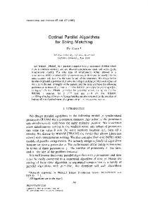
An example input instance with optimal solutions for different values of d is shown in Figure 1. We call val(A) the value of A. Observe that d can also be negative: in that case, matching a white gene to two black genes is penalized instead of encouraged, which might be useful, for example to avoid that the number of matched white genes is too low. Moreover, in the above model, any information about the similarity of genes in B is ignored. A natural extension of this model is thus to incorporate knowledge about genes from the duplicated genome. More precisely, we can assume that the graph G contains, for each pair of black vertices, an edge if the corresponding genes are likely to be in-paralogs. Using a maximum-parsimony approach, the aim is then to identify clusters of orthologs that minimize the total weight of the edges between clusters as these contradict the orthology groups. Equivalently, we aim at finding clusters that maximize the weight of edges within the sought clusters. For the formal problem definition, first observe that, in this second model, the input graph is not bipartite anymore. Second, we need to define the set of allowed groups of orthologs. For this, from now on, let the term cluster denote a (connected) subgraph of G that contains at least one edge. Since the overall aim is still to find orthology relations between the white and black vertices, the clusters we allow in our model must contain only one white vertex, and must be connected to at least one and at most two black vertices. Among such possible clusters, we allow only three types, that we will call ortholog clus5
0404520
0413290
1576920
1526790
0016s04980 0006s05760 0001s05340 0003s22060 0001s27820 0009s07000 0404520
0413290
1576920
1526790
0016s04980 0006s05760 0001s05340 0003s22060 0001s27820 0009s07000 0404520
0413290
1576920
1526790
0016s04980 0006s05760 0001s05340 0003s22060 0001s27820 0009s07000 0404520
0413290
1576920
1526790
0016s04980 0006s05760 0001s05340 0003s22060 0001s27820 0009s07000 Figure 1: An example instance of OAD. The first row shows a connected component of the graph for Ricinus communis and Populus trichocarpa; white vertices represent ricinus genes, black vertices represent poplar genes, and (for simplicity) edges have unit weight. The second row shows an optimal solution to standard matching. The third row shows an optimal solution with duplication bonus d = 0. The fourth row shows an optimal solution with duplication bonus d > 0. The vertex names are the identifiers from the corresponding data sets in the CoGe database (https://genomevolution.org/coge).
ters: (i) one white and one black vertex connected by an edge, (ii) a path of length two where the middle vertex is white, and (iii) triangles with exactly one white vertex. Observe that in particular, we exclude the possibility of having an ortholog group in which the white vertex is considered dissimilar to one of the two black vertices. In a similar way as Orthology Assignment with Duplications, we can now formally define the Orthology Clustering with Duplications problem. Orthology Clustering with Duplications (OCD) Instance: An undirected graph G = (W ] B, E), an edge-weight function s : E → Q+ . Task: Find a partition (C1 , . . . , C` , I) of W ] B into ortholog clusters C1 , . . . , C` and isolated vertices I such that val(C1 , . . . , C` , I) := P` P i=1 a⊆Ci s(a) is maximized. Note that the duplication bonus d used in the definition of Orthology Assignment with Duplications is not necessary in this model, as it can be incorporated in the input graph, by adding d to every edge weight for all edges of G connecting pairs of black vertices having at least one common neighbor— 6
if such an edge does not exist in G, then we may create it and assign it the weight d. We consider in this paper only simple undirected graphs G = (V, E) where the vertex set V has two disjoint subsets, a set W of white vertices and a set B of black vertices. We use n := |W | + |B| to denote the number of vertices and m := |E| to denote the number of edges in the input graph. For a vertex v in G, NG (v) denotes the set of neighbors of v in G. Our analysis of OCD is in the context of parameterized complexity, where we analyze the running time of algorithms for NP-hard problems not only with respect to the input size, but also secondary parameters. Herein we try to encapsulate the combinatorial explosion in a function of the parameter. See a recent textbook [22] for more context and methodology. 3. Polynomial-Time Algorithms for Finding Orthologs in Two Genomes In this section, we provide polynomial-time algorithms for Orthology Assignment with Duplications. First, we consider the (simpler) case in which there there is no duplication bonus, or there is a duplication penalty. Theorem 1. Orthology Assignment with Duplications can be solved √ in O( n · m) time if d ≤ 0. Proof. Construct a graph G0 from the input graph G as follows. First add all black vertices of G to G0 . Then replace each white vertex w by two white copies w1 , w2 such that NG (w) = NG0 (w1 ) = NG0 (w2 ). The edge weights between w1 and NG (w) are the same as the edge weights between w and NG (w), that is, for each b ∈ NG (w), s({w1 , b}) := s({w, b}). For w2 , we add d to these edge weights, that is, s({w2 , b}) := s({w, b}) + d (recall that d ≤ 0). We will compute an optimal orthology assignment by computing a maximumweight matching in G0 . To this end, we now show that G has an orthology assignment with duplications of value at least ` if and only if G0 has a matching of weight at least `. First, let A be an orthology assignment with duplications in G of value at least `. Construct an edge set M of G0 by adding for each vertex w ∈ W the following edges. If w is incident with two edges {w, b1 } and {w, b2 } of A, then add {w1 , b1 } and {w2 , b2 } to M . If w is incident with exactly one edge {w, b} of A then add {w1 , b1 } to M . The edge set M is independent and the sum of the edge weights is exactly the sum of the weights of A plus d times the number of white vertices that are incident with two edges of A. Hence, the weight of the matching is the same as the value of A, as claimed. Conversely, let M be a matching of weight at least ` in G0 . Without loss of generality, let M be a maximum-weight matching. Consider the set A of edges of G that contains for each vertex w ∈ W and each vertex b ∈ B, the edge {w, b} if and only if either {w1 , b} ∈ M or {w2 , b} ∈ M . Then, each black vertex is incident with at most one edge in A and each white vertex is incident with at 7
most two edges in A. Hence, A is an orthology assignment with duplications. Moreover, since M has maximum weight, M contains an edge incident with w2 only if it contains an edge incident with w1 . Thus, for each white vertex w ∈ W , there is exactly one edge incident with w in A if and only if M contains an edge that is incident with w1 and M does not contain an edge incident with w2 . Then, the contribution of each w to A is exactly the same as the contribution of the edges that are incident with w1 and w2 to M : If M has only an edge incident with w1 , then the weights of the two edges in M and A are the same and w does not contribute to the second part of the value sum. Otherwise, the contribution of w to A is s(w, b1 ) + s(w, b2 ) + d = s(w1 , b1 ) + s(w2 , b2 ). The proof of the second direction of the equivalence describes a linear-time algorithm for constructing an assignment from a matching in G0 . Hence, we can find an optimal assignment by first computing the graph G0 , then computing a maximum-weight matching in G0 and then computing an assignment from this matching. The overall running time is dominated by the time needed to compute the matching. √Since G0 has O(n) vertices and O(m) edges, this step can be performed in O( n · m) time [23]. We now turn to the case where d > 0. Theorem 2. Orthology Assignment with Duplications can be solved √ in O( n · m) time if d > 0. Proof. Construct a graph G0 from the input graph G as follows. First, add all black vertices of G to G0 . Then, replace each white vertex w by two copies w1 , w2 such that, initially NG (w) = NG0 (w1 ) = NG0 (w2 ). The weights of these edges are obtained from the old ones by adding a value of d each time, that is, s({w1 , b}) := s({w, b}) + d and s({w2 , b}) := s({w, b}) + d. Further, for each pair w1 , w2 of new white vertices that correspond to the same white vertex in W , add the edge {w1 , w2 } to G0 and assign a weight of d to it. We will compute an optimal orthology assignment by computing a maximumweight matching in G0 . To this end, we now show that G has an orthology assignment with duplications of value at least ` if and only if G0 has a matching of weight at least ` + d · |W |. First, let A be an orthology assignment for G of value at least `. Construct a matching M as follows. Consider each w ∈ W . If w is incident with two edges {w, b1 } and {w, b2 } in A, then add the edges {w1 , b1 } and {w2 , b2 } to M . If w is incident with exactly one edge {w, b} of A, then add the edge {w1 , b} to M . If w is not incident with any edge of A, then add the edge {w1 , w2 } to M . In order to compare the value of A with the weight of M , we now consider each white vertex of G separately. Case 1: w is not incident with any edge of A. Then, the contribution of w to val(A) is zero. By construction, M contains the edge {w1 , w2 }. Thus, the edges incident with w1 and w2 contribute exactly d to the weight of M .
8
Case 2: w is incident with exactly one edge {w, b} of A. Then, the contribution of w to val(A) is s({w, b}). Due to construction of M , only w1 is incident with an edge of M . The weight of this edge is s({w, b}) + d. Case 3: w is incident with two edges {w, b1 } and {w, b2 } of A. Then, the contribution of w to val(A) is s({w, b1 }) + s({w, b2 }) + d. Due to construction of M , w1 and w2 are incident with edges of M , one having b1 as endpoint and one having b2 as endpoint. The weights of these edges are s({w, b1 }) + d and s({w, b2 }) + d, respectively. In each case, the contribution of w to val(A) is d less than the contribution of w1 and w2 to the weight of M . Thus, the weight of M is at least val(A)+d·|W |, as claimed. Conversely, let M be a matching of weight at least ` + d · |W | in G0 . Without loss of generality, assume that M is a maximum-weight matching. Consider the set A of edges of G that contains for each vertex w ∈ W and each vertex b ∈ B, the edge {w, b} if and only if either {w1 , b} ∈ M or {w2 , b} ∈ M . We compare again the weight of M with the value of A. We do this by grouping the contributions of the white vertices in G0 in the pairs w1 , w2 . First, observe that, since M is a maximum-weight matching, at least one of w1 or w2 is incident with an edge in M ; otherwise, adding {w1 , w2 } to M gives a matching with higher weight. Moreover, we can assume without loss of generality, that it is w1 that is always incident with an edge of M . Thus, it is sufficient to consider the following three cases. Case 1: only w1 is incident with an edge {w1 , b} of M . Then, the contribution of w1 to the weight of M is s({w, b}) + d. By construction, A contains the edge {w, b} and no other edge incident with w. Thus, the contribution of w to val(A) is s({w, b}) and therefore d less than the contribution of w1 and w2 to M . Case 2: M contains {w1 , w2 }. Then, the contribution of w1 and w2 to M is d. By construction, w is not incident with any edge of A. Thus, the contribution of w to val(A) is zero and therefore d less than the contribution of w1 and w2 to M . Case 3: M contains {w1 , b1 } and {w2 , b2 }. Then, the contribution of w1 and w2 to M is s({w, b1 })+d+s({w, b2 })+d. By construction, w is incident with two edges of A: the edge {w, b1 } and the edge {w, b2 }. Thus, the contribution of w to val(A) is s({w, b1 }) + s({w, b2 }) + d and therefore it is d less than the contribution of w1 and w2 to M . In each case, the contribution of w to the value of A is exactly d less than the contribution of w1 and w2 to the weight of M . Thus, the value of A is at least ` + d · |W | − d · |W | = `, as claimed. Thus, a maximum-weight matching in G0 directly corresponds to an optimal assignment in G. Moreover, the second part of the proof gives a linear-time algorithm for computing such an assignment from the maximum-weight matching. Hence, we can find an optimal assignment by first computing the graph G0 , then computing a maximum-weight matching in G0 and then computing an assignment from this matching. The overall running time is dominated by the time needed to compute the matching. Since G0 has O(n) vertices and O(m) edges, 9
√ this step can be performed in O( n · m) time [23]. Finally, let us remark that the problem of computing a maximum-weight matching in a bipartite graph can be easily reduced to Orthology Assignment with Duplications with d = 0: Pick an arbitrary part of the vertex bipartition to be the white part of the Orthology Assignment with Duplications instance and add for each vertex v of this part a further vertex that has only v as neighbor and assign a sufficiently large weight to this edge. Then, any assignment will include these new edges and further edges of the assignment directly correspond to a maximum-weight matching of the original bipartite graph. A similar construction works if d > 0. Hence, any faster algorithm for Orthology Assignment with Duplications would directly imply a faster algorithm for computing maximum-weight matchings. 4. Including Similarities in the Duplicated Genome Makes it Hard We now consider the more general problem where the score of an orthology group may also take information between genes of the duplicated genome into account. Unfortunately, this extension of the model results in a computationally hard problem. The reduction we use to prove NP-hardness is similar to a known NP-hardness reduction for the Cluster Editing problem [24]. Theorem 3. Orthology Clustering with Duplications is NP-hard, even when the input graph has maximum degree six and weights are all unitary. Proof. The reduction is from the 3-SAT problem where we have a Boolean formula φ in conjunctive normal form and clauses of size exactly three and we ask whether φ is satisfiable. Let N be the number of variables in φ and M the number of its clauses. Denote the maximum number of occurrences of a variable in any clause by `. (Without loss of generality, we assume that each variable occurs only once in each clause.) We show how to construct in polynomial time a white/black-colored graph G which admits a set of vertex-disjoint ortholog clusters containing at least 3`N edges if and only if φ is satisfiable. This directly implies the NP-hardness of Orthology Clustering with Duplications. Let us construct G, which is the empty graph initially. First, add N cycles, each with 2` black vertices, corresponding to the variables in φ. For each cycle, label the edges in an arbitrary maximum matching by positive and the remaining edges by negative. This labeling is used only in the construction and will not be part of the final instance. Next, for each clause, add a white vertex v and attach it to the cycles of the variables it contains as follows. For each positive literal x, make v adjacent to the two endpoints of a positive edge of the cycle of x. For each negative literal ¬x, make v adjacent to the endpoints of a negative edge of the cycle of x. For each of these connections, choose an edge whose endpoints are not yet connected to any clause vertex. Note that this is always possible since each cycle has length 2`. Finally, introduce `N − M white dummy vertices that are connected to each vertex in each cycle. (Note that M ≤ `N/3, so this is possible.) We assign each edge weight one, meaning that the value of a 10
clustering is simply the number of edges contained in its clusters. This concludes the construction of G. As indicated above, we ask for an ortholog clustering of at least 3`N edges. Now assume that φ is satisfiable and fix an arbitrary satisfying assignment of the variables. Hence, for each clause there is a literal satisfying this clause. To construct a clustering for G, for each clause C, we pick as a ortholog cluster a triangle in G which consists of the white vertex corresponding to the clause and the endpoints of an edge in a variable cycle. The variable is chosen such that its literal in C is satisfied, that is, if the literal is positive, then the edge in the triangle is positive and vice versa. Note that we can indeed pick these clusters, because, first, by the way we connected the clause vertices and variable cycles, no positive (resp. negative) edge blocks another positive (resp. negative) edge from being taken into a cluster, and, second, because choosing the clusters in this way, we consistently choose only positive or only negative edges from each variable cycle. Hence, we obtain M clusters with three edges each. Finally, for each variable cycle, we complete the set of cluster edges in it to a perfect matching, by making all remaining matching edges into a cluster with an arbitrary dummy vertex. In total, we obtain M + `N − M = `N ortholog clusters, each with three edges. That is, the Orthology Clustering with Duplications instance has a solution. Now assume that G has a set of ortholog clusters with at least 3`N edges overall. Observe that G contains exactly `N white vertices and thus, at least `N edges inside the ortholog clusters are between black vertices. Since in each of the N variable cycles there are at most ` edges in clusters, and these are the only “black” edges, the clusters induce perfect matchings in each variable cycle. Thus, for each cycle, the edges correspond to a valid assignment of truth values to the variables: Assign each variable x in φ the value true if the cluster edges from the corresponding cycle are positive and assign it false, otherwise. Since there are only `N − M white dummy vertices, all M clause vertices are in ortholog clusters. By the way in which we connected the clause vertices to the variable cycles, this means that each clause is satisfied by φ. The NP-hardness of OCD motivates fixed-parameter algorithms for this problem. Observe that OCD can be viewed as an edge deletion problem: delete a minimum-weight set of edges such that only the edges of the ortholog clusters Ci remain. The standard parameter for such problems is the number of edge deletions k to obtain a solution [25, 26]. It is easy to obtain fixed-parameter tractability for OCD and parameter k as the following shows. Proposition 1. Let (G = (V, E), s) be an instance of OCD such that no connected component is an ortholog cluster, let (C1 , . . . , C` , I) be an ortholog clustering of G, and let k denote the number of edges not contained in any ortholog cluster Ci . Then, |E| ≤ 7k. Proof. In an instance as described above, every ortholog cluster is incident with at least one edge deletion. Thus, the number of ortholog clusters is at most 2k. Since an ortholog cluster has at most three edges, this implies that such a graph 11
has at most 7k edges: at most 6k edges in the ortholog clusters and at most k deleted edges. The above proposition shows that k is not a small parameter. In order to obtain more efficient fixed-parameter algorithms, we consider two smaller parameters. The first parameter is as follows. Definition 2 (Parameter kB ). Given an instance of OCD, by kB we denote the number of edge deletions necessary to destroy all paths on three vertices that start and end with a white vertex. Clearly, such paths cannot be contained completely in any ortholog cluster Ci . Hence, kB ≤ k. The second parameter is defined below. Definition 3 (Parameter kW ). Given an instance of OCD, by kW we denote the number of edge deletions necessary to destroy all subgraphs containing a white vertex with degree three. In an ortholog cluster, every white vertex has degree at most two. Hence, kW ≤ k. A further P advantage of kB and kW is that they can Pbe easily computed as in fact kB = b∈B max{|N (b) ∩ W | − 1, 0} and kW = w∈W max{|N (w)| − 2, 0} (recall that white vertices have only black neighbors). Hence, one may easily decide whether kB or kW are small, and thus whether they are appropriate parameters. In the following, we say that a reduction rule is correct if the objective value of an optimal solution is the same before and after the rule is applied. Similarly, a branching rule is correct if the optimal solution of one of the recursive branches gives an optimal solution of the instance to which the rule is applied. A fixed-parameter algorithm for kB . We first describe a search tree algorithm for parameter kB . The strategy of the algorithm is to first destroy all paths between white vertices. Branching Rule 4. If B contains a vertex b with at least two neighbors w1 , w2 ∈ W , branch into the two cases to delete either {b, w1 } or {b, w2 }. The branching rule is correct since any ortholog cluster can contain at most one of {b, w1 } and {b, w2 }. In the recursive branches, parameter kB is decreased by at least one. Moreover, if kB = 0, the rule does not apply. Since this is the only branching rule that we apply, this implies that the resulting search tree has size O(2kB ). We now show that all instances for which the rule does not apply can be solved in linear time by applying two reduction rules. Reduction Rule 5. If G contains an edge {b1 , b2 } such that b1 , b2 ∈ B do not have a common neighbor in W , then delete {b1 , b2 }. Reduction Rule 6. If G contains a connected component G0 that is not an ortholog cluster and has exactly one white P vertex w, then compute an ortholog cluster C such that C contains w and a⊆C s(a) is maximum. Delete all edges of G0 that are not contained in C. 12
Lemma 1. Reduction Rules 5 and 6 are correct and can be executed exhaustively in O(m + n) time. Proof. Reduction Rule 5 is correct since no such edge {b1 , b2 } can be part of an ortholog cluster. It can be applied exhaustively in O(m + n) time since every vertex in B has at most one neighbor in W (because Branching Rule 4 does not apply by hypothesis). The correctness of Reduction Rule 6 is implied by two facts. First, any ortholog cluster containing a vertex from G0 contains w. Second, in any optimal solution, any vertex of G0 is either contained in an ortholog cluster with w or belongs to the set I of isolated vertices. The running time can be seen as follows. Say that a connected component C of G is amenable if it fulfills the condition of Reduction Rule 6, that is, C is not an ortholog cluster and contains exactly one white vertex. First, in O(m + n) time, we compute the amenable connected components of G. Then, for each such connected component do the following. If w has only one neighbor b in G0 , then {w, b} is the optimal cluster C and we are done. Otherwise, we first find the two edges incident with w that have the largest two edge weights. The sum of these two edge weights gives the best ortholog cluster among those that do not contain an edge between the two black vertices. Thus, initialize C with the three corresponding vertices. Then, for each edge e incident with two black vertices b1 and b2 , we check whether the endpoints of the edge are both adjacent to w. If this is the case, then compute in O(1) time the sum s(b1 , b2 )+s(b1 , w)+s(b2 , w). If this sum exceeds the sum of the edges in the current best ortholog cluster C, then update C accordingly. Clearly, this procedure computes the optimal ortholog cluster C for each amenable connected component. All edges not contained in any such cluster C but in amenable connected components can be deleted in linear time. Now the overall running time follows from the fact that deleting edges in amenable connected components does not create new amenable connected components. Theorem 7. Orthology Clustering with Duplications can be solved in O(2kB · (m + n)) time. Proof. The algorithm first applies Branching Rule 4 as long as possible. Afterwards, in each leaf of the corresponding search tree, it applies Reduction Rules 5 and 6 exhaustively. In the remaining instance all connected components are ortholog clusters and we can compute the value of the corresponding clustering by computing the sum of the edge weights in the graph associated with the leaf of the search tree. By keeping the best clustering found in any leaf, the algorithm computes an optimal solution. As argued above, the search tree produced by the algorithm has size O(2kB ). Hence, the running time bound can be obtained by showing that in each search tree node, we spend O(m + n) time. Clearly, we can check in O(m + n) time whether Branching Rule 4 applies. By Lemma 1, Reduction Rules 5 and 6 can be applied exhaustively in O(m + n) time. Finally, if these rules do not 13
apply, then the value of the ortholog clustering is computed by summing all edge weights in O(m + n) time. A fixed-parameter algorithm for kW . The approach is again to first destroy all subgraphs containing a white vertex of degree at least three via branching. Instances that do not contain such a vertex are solved by computing a maximumweight matching in an auxiliary graph. Branching Rule 8. If B contains a vertex w ∈ W with at least three neighbors b1 , b2 , b3 ∈ B, branch into the three cases to delete either {w, b1 }, {w, b2 }, or {w, b3 }. The correctness follows from the fact that in every ortholog cluster, the white vertex has degree at most two. Lemma 2. Let (G, s) be an instance of Orthology Clustering with Duplications such that √ every vertex in W has degree at most two. Then, (G, s) can be solved in O( n · m) time. Proof. First, apply Reduction Rule 5 exhaustively to G; this can be done in O(m + n) time. Afterwards, construct an auxiliary graph G0 with edge weight function s0 derived from G and s as follows. The graph G0 is obtained from G by adding an edge between all black vertices that have a common white neighbor. Observe that by the condition of the lemma, each white vertex has at most two neighbors. Thus, the number of added edges is O(n). Then, for every edge {b1 , b2 } between two black vertices in G0 that share at least one common white neighbor, carry out the following operation. Let w ∈ W be a common neighbor such that s(b1 , w) + s(b2 , w) is maximum. Then, set s0 (b1 , b2 ) := s(b1 , b2 ) + s(b1 , w) + s(b2 , w) if {b1 , b2 } is contained in G and s0 (b1 , b2 ) := s(b1 , w) + s(b2 , w), otherwise. Intuitively, this means that the new weight of {b1 , b2 } records not only the similarity between b1 and b2 but instead the weight of the best ortholog cluster that contains b1 and b2 . For all other edges set s0 (a) := s(a). We now show that the best ortholog clustering in (G, s) corresponds to a maximum-weight matching in (G0 , s0 ). More precisely, we show that (G, s) has an ortholog clustering of value ` if and only if (G0 , s0 ) has a matching of weight `. First, let (C1 , . . . , C` ) be an ortholog clustering of value `. Construct a matching M in (G0 , s0 ) as follows: For each cluster Ci consisting of exactly two vertices b and w add the edge {b, w} to M . For each cluster Ci containing three vertices b1 , b2 , and w where b1 , b2 ∈ B add the edge {b1 , b2 } to M . By definition, the sum of the edge weights of M in G0 is at least `. Moreover, M is a matching since the Ci s have disjoint vertex sets. For the converse direction, we mainly have to prove that clusters corresponding to matching edges are pairwise vertex disjoint. If a matching edge e ∈ M is between two black vertices b1 , and b2 , then let w be the vertex such that s(b1 , w) + s(b2 , w) is maximum. Construct an ortholog cluster C containing b1 , b2 , and w and the edges between them. The weight of the edges of C in G
14
is, by definition of s0 , exactly s0 (b1 , b2 ). If a matching edge e ∈ M is between a black and a white vertex, then construct an ortholog cluster containing the endpoints of e and u. Again by definition of s0 , the weight of the edge e in G0 and the value of the ortholog cluster in G are the same. It remains to show that no two ortholog clusters have a vertex in common. The only possibility for a vertex to be in two ortholog clusters occurs when a white vertex w is added to a matching edge {b1 , b2 } to produce a cluster. By the condition of the lemma, vertex w has no further neighbors in G0 and thus the pair {b1 , b2 } is the only pair that may cause an addition of w to a cluster. Thus, the produced set of vertex sets is an ortholog clustering of weight `. Observe that the converse direction of the proof also describes a linear-time algorithm to construct an optimal ortholog clustering from a maximum-weight matching in G0 . The overall running time bound follows from the fact that G0 can be constructed in O(n + m) time and has n vertices and O(m) edges. We immediately obtain the following running time bound on the search tree algorithm by observing that Branching Rule 8 produces a search tree of size O(3kW ). Theorem √ 9. Orthology Clustering with Duplications can be solved in O(3kW · n · m) time. 5. Experiments In the following, we report on our empirical findings for the Orthology Assignment with Duplications (OAD) and Orthology Clustering with Duplications (OCD) models and the algorithms developed for them in Sections 3 and 4. Data Acquisition. We built instances based on the genomes of Ricinus communis [27] (castor bean), Populus trichocarpa [28] (western balsam poplar), and Theobroma cacao [29] (cacao tree). Of these three species, Populus trichocarpa has undergone a whole genome duplication after the speciation events. Accordingly, we built one set of instances with Ricinus communis as white species and one set of instances with Theobroma cacao as white species; Populus trichocarpa is the black species in both sets. In the following, we refer to the three species as Ricinus, Cacao, and Populus. To build the graphs, following the methodology introduced previously [5, 9], we computed BLAST Expect (E) values [30] which measure the expected number of hits with the same alignment score that would be encountered in a random string of the same size. We add an edge between two genes if the E-value is below some threshold. We use three threshold values t ∈ {0.0, 10−140 , 10−80 }. Each edge in the built graphs has weight one. To keep the size of the OCD instances reasonable, we use an explicit duplication bonus d instead of creating edges between all pairs of black vertices as described in Section 1 (which is equivalent in the unweighted case).
15
Table 1: Some general properties of the instances for OAD and OCD. Here, nB is the number of black vertices, nW the number of white vertices, and mOAD and mOCD the number of edges in the OAD and OCD instances, respectively. By n∗ we denote the order of the largest component and with n | 95 the 95th percentile of the component orders, and analogously we denote the maximum and 95th percentile values of kB and kW . Ricinus vs. Populus
Cacao vs. Populus
t
10−80
10−140
0.0
10−80
10−140
0.0
nB nW n∗ n | 95 mOAD mOCD # comp. # nontr. comp # diff. comp ∗ kB ∗ kW kB | 95 kW | 95
24472 15111 1914 12 132446 269862 7980 2493 2141 30351 30608 20 20
18079 11333 316 10 56438 109352 7102 1897 1620 2848 2895 13 12
14235 9075 201 9 34445 64162 6247 1504 1272 1268 1327 8 8
25165 16963 2261 13 227778 368430 7847 2698 2373 65613 65300 25 24
18140 12488 440 11 77887 131568 7043 2008 1806 5957 5946 15 13
14287 9907 256 9 44251 73837 6152 1613 1456 3723 3723 11 9
Implementation Details. The algorithms were implemented in Python 2.7.6 using NetworkX 1.11.5 For OAD, we used a straightforward implementation of the algorithms described in Section 3. For OCD we implemented the fixedparameter algorithm for parameter kB since numerical evaluation showed that the search tree size for this parameter was usually smaller than for kW . To improve the running time, apart from Reduction Rules 5 and 6, we implemented further reduction rules related to situations in which vertices’ neighbors are subsets of other vertices’ neighbors and where the optimal matches of a white vertex can be determined locally. If kW = 0 during the execution of the algorithm, then we use the algorithm from Lemma 2 to solve the remaining instance. Instance Properties. Some general instance properties and statistics about the results for OAD are shown in Table 1. As the table shows, the graphs decompose into a large number of smaller connected components, most of which are trivial, that is, they consist of one white vertex and one or two black vertices. The largest connected components contain between 201 and 1914 vertices. The majority of the nontrivial components have at most 10 vertices. Similarly, for the majority of nontrivial components, the two parameters kB and kW have moderate values. Note also that the size of the instances, in terms of the number of edges, increases roughly twofold between each increment of the threshold value. Each edge between two black genes represents a possible paralog. These possible paralogs are taken into account in the OCD instances and not in the OAD instances. They make up roughly half of the edges in the OCD instances. Solution Statistics for OAD and OCD. We computed the solutions for OAD and OCD for the instances described above. For OCD, not all connected com5 Source
code and results are available at http://fpt.akt.tu-berlin.de/oad.
16
Table 2: Number and type of the clusters output for OAD and OCD. Here, d is the duplication bonus, C is the total number of clusters, B is the number of covered black genes, and %{P2 , P3 , K3 } is the number of the clusters of the corresponding type. OAD d
C
B
OCD
%P2
%P3
%K3
C
B
%P2
%P3
%K3
51.94 39.75 39.35 39.22
0.00 1.44 1.70 1.82
48.06 58.81 58.95 58.96
12994 13082 13082 13080
53.65 43.44 42.99 42.77
0.00 1.26 1.55 1.71
46.35 55.30 55.46 55.52
11319 11379 11378 11379
54.59 45.44 44.92 44.61
0.00 0.91 1.28 1.52
45.41 53.65 53.80 53.87
15195 15349 15345 15344
53.51 39.80 38.71 38.45
0.00 2.10 2.86 3.11
46.49 58.10 58.43 58.44
12996 13075 13073 13071
56.24 43.81 43.27 42.99
0.00 1.22 1.61 1.84
43.76 54.98 55.13 55.17
11301 11357 11352 11352
56.64 45.15 44.56 44.34
0.00 1.04 1.47 1.70
43.36 53.82 53.98 53.96
Ricinus vs. Populus, t = 10−80 -1.1 -0.5 0.0 1.0
14811 14811 13826 13293
14811 22724 22724 22724
100.00 46.57 35.64 29.05
0.00 6.41 7.83 9.10
0.00 47.01 56.53 61.85
10274 9571 9547 9539
15212 15338 15337 15337
Ricinus vs. Populus, t = 10−140 -1.1 -0.5 0.0 1.0
11085 11085 10547 10216
11085 16756 16756 16756
100.00 48.84 41.13 35.98
-1.1 -0.5 0.0 1.0
8873 8873 8498 8258
8873 13228 13228 13228
100.00 50.92 44.34 39.82
0.00 4.97 5.87 6.60
0.00 46.19 53.00 57.42
8879 8356 8332 8319
Ricinus vs. Populus, t = 0.0 0.00 3.87 4.28 5.16
0.00 45.22 51.38 55.03
7784 7362 7337 7323
Cacao vs. Populus, t = 10−80 -1.1 -0.5 0.0 1.0
16154 16154 14624 13913
16154 24048 24048 24048
100.00 51.13 35.56 27.15
0.00 7.69 10.84 12.86
0.00 41.17 53.60 59.99
10373 9581 9514 9498
Cacao vs. Populus, t = 10−140 -1.1 -0.5 0.0 1.0
11887 11887 10960 10514
11887 17371 17371 17371
100.00 53.87 41.51 34.78
-1.1 -0.5 0.0 1.0
9469 9469 8802 8502
9469 13708 13708 13708
100.00 55.23 44.26 38.77
0.00 4.59 6.51 8.07
0.00 41.54 51.98 57.14
9040 8371 8341 8325
Cacao vs. Populus, t = 0.0 0.00 3.89 4.79 5.80
0.00 40.88 50.94 55.43
7883 7334 7303 7293
ponents could be solved within reasonable time as our algorithms have exponential running times in the worst case. Hence, we set a timeout of 60 seconds for each connected component. With this setting, the connected components solved by OCD contained altogether between a minimum of 63% of the vertices (attained for Cacao and t = 10−80 ) and a maximum of 87% (for Ricinus and t = 0.0), and the total running time for an instance of OCD ranged between 2.1 and 6.7 hours. In contrast, all OAD instances could be solved in reasonable time, with the largest instance taking 2 minutes. Table 2 shows solution statistics for OAD and OCD for different values of the duplication bonus d and the distribution of the ortholog clusters into P2 -clusters (single edges), P3 -clusters (a white vertex with two black neighbors that are not adjacent in the OCD instance), and K3 -clusters (a white vertex and two black vertices, pairwise adjacent in the OCD instance). Observe that,
17
Table 3: Number and type of the clusters output for OAD and OCD restricted to components that were solved by both methods. Here, d is the duplication bonus, C is the total number of clusters, B is the number of covered black genes, and %{P2 , P3 , K3 } is the number of the clusters of the corresponding type. OAD d
C
B
OCD
%P2
%P3
%K3
C
B
%P2
%P3
%K3
51.94 39.75 39.35 39.22
0.00 1.44 1.70 1.82
48.06 58.81 58.95 58.96
12994 13082 13082 13080
53.65 43.44 42.99 42.77
0.00 1.26 1.55 1.71
46.35 55.30 55.46 55.52
11319 11379 11378 11379
54.59 45.44 44.92 44.61
0.00 0.91 1.28 1.52
45.41 53.65 53.80 53.87
15195 15349 15345 15344
53.51 39.80 38.71 38.45
0.00 2.10 2.86 3.11
46.49 58.10 58.43 58.44
12996 13075 13073 13071
56.24 43.81 43.27 42.99
0.00 1.22 1.61 1.84
43.76 54.98 55.13 55.17
11301 11357 11352 11352
56.64 45.15 44.56 44.34
0.00 1.04 1.47 1.70
43.36 53.82 53.98 53.96
Ricinus vs. Populus, t = 10−80 -1.1 -0.5 0.0 1.0
10274 10274 9819 9527
10274 15345 15345 15345
100.00 50.64 43.72 38.93
0.00 3.66 4.25 4.66
0.00 45.70 52.03 56.41
10274 9571 9547 9539
15212 15338 15337 15337
Ricinus vs. Populus, t = 10−140 -1.1 -0.5 0.0 1.0
8879 8879 8534 8304
8879 13082 13082 13082
100.00 52.66 46.71 42.46
0.00 2.95 3.48 3.96
0.00 44.39 49.81 53.58
8879 8356 8332 8319
Ricinus vs. Populus, t = 0.0 -1.1 -0.5 0.0 1.0
7784 7784 7505 7312
7784 11382 11382 11382
100.00 53.78 48.34 44.34
0.00 2.62 2.97 3.62
0.00 43.60 48.69 52.04
7784 7362 7337 7323
Cacao vs. Populus, t = 10−80 -1.1 -0.5 0.0 1.0
10373 10373 9821 9485
10373 15352 15352 15352
100.00 52.00 43.68 38.14
0.00 4.85 5.85 6.49
0.00 43.15 50.46 55.36
10373 9581 9514 9498
Cacao vs. Populus, t = 10−140 1.1 -0.5 0.0 1.0
9040 9040 8580 8318
9040 13080 13080 13080
100.00 55.31 47.55 42.75
-1.1 -0.5 0.0 1.0
7883 7883 7486 7291
7883 11360 11360 11360
100.00 55.89 48.25 44.19
0.00 2.75 3.52 4.24
0.00 41.94 48.93 53.01
9040 8371 8341 8325
Cacao vs. Populus, t = 0.0 0.00 2.87 3.09 3.69
0.00 41.24 48.66 52.12
7883 7334 7303 7293
while the OAD instances contain no edges between black vertices, we use these edges to compute the cluster distribution. Using OAD, the ratio of white genes covered by clusters ranges between 82 % and 98 % over all instances, threshold values, and duplication bonuses. The coverage of black genes ranges between 92 % and 95 % for duplication bonuses between −0.5 and 1.0, and around 60 % if the bonus is −1.1. Indeed, for OAD with d = −1.1 we obtain the same solutions that we would obtain by computing a maximum matching between the white and black genes. In contrast, for OCD with d = −1.1 we see a sharp divide into clusters of size two and K3 -clusters. OCD failed to solve larger components; Table 3 compares OAD and OCD on those components that were solved by both variants. Extrapolating from these data, OCD covers a similar ratio of black and white genes as OAD, except for
18
the case of black genes and duplication bonus −1.1: The coverage of black genes for OCD with duplication bonus −1.1 does not differ substantially from the one for other duplication bonuses. Generally, we see that higher duplication bonus leads to a lower number of clusters meaning less coverage for the set of white genes. Observe that, somewhat counterintuitively, the percentage of K3 -clusters is sometimes higher for OAD although OAD ignores these edges. The reason for this is simply that OCD failed to solve the larger components which contain more potential paralogs: The comparison of the OCD results to the OAD results restricted to the components that were solved by OCD in Table 3 shows that OCD always identifies more K3 -clusters. Notably, the number of P3 -clusters identified by the OCD model is at most half the one for OAD. Similarly to the number of K3 -clusters, it may seem that the number of covered black genes is much lower for OCD, but Table 3 reveals that the coverage is only marginally smaller when restricted to the components both algorithms could solve. In summary, we see that OAD and OCD cover in ortholog clusters large ratios of both black and white genes, regardless of the threshold t. The coverage between the two methods is similar, barring computational barriers, except for duplication bonus −1.1, where it is significantly lower for OAD. In contrast to OAD, OCD produces roughly half the number of P3 -clusters and slightly more K3 -clusters. Similarity of Predicted Paralogs for OAD and OCD. The solution statistics show that both OAD and OCD identify large numbers of supposed orthologs. We now evaluate the biological quality of these results using three tests. Recall that the clusters of size three for OAD and OCD are in fact predictions of pairs of paralogs in the duplicated genome. In our case, this is the Populus genome. It is expected that paralogs have high sequence similarity. In the first test, we thus evaluate the Blast E-values of the predicted paralogs. Moreover, we expect that the sequence similarity for the predicted paralogs of Populus is higher than both sequence similarities between the Populus genes and the Ricinus or Cacao genes. In other words, we expect that the gene tree of the three sequences in the cluster agrees with the species tree of the two species. We check whether this is indeed the case in the second test, a standard test in comparative genomics. As the third and final test, for each pair of predicted paralogs, we retrieved and compared their chromosome number. Paralogs that arise due to the genome duplication event should be located on different chromosomes. Hence, we computed the percentage of paralogs that are located on different chromosomes. We expect that a higher percentage indicates a higher percentage of correctly assigned paralogs. Among the matched genes, in general, smaller threshold values lead to larger percentages for correct gene trees regardless of which of the two methods we use. For OAD the number of output clusters with correct gene trees range between at least 50 % and at least 90 % with increases of circa 20 % per decrement of 19
Table 4: Average sequence similarity for the predicted paralogs and percentage of clusters for which the gene tree matches the sequence tree using the OAD model. Here d denotes the duplication bonus and e | x the BLAST E-value at the xth percentile, % cgt denotes the percentage of size-three clusters with correct gene trees, % dc denotes the percentage size-three clusters whose predicted paralogs are located on different chromosomes of Populus. d −1.1 −0.5 0.0 1.0
e | 75
e | 50
e | 25
% cgt
% dc
Ricinus vs. Populus, t = 10−80 — — — — 3.35e-112 2.91e-161 0.00e+00 61.03 2.48e-111 5.32e-159 0.00e+00 60.46 4.43e-110 3.43e-157 0.00e+00 59.66
— 83.89 83.56 83.52
Ricinus vs. Populus, t = 10−140 −1.1 −0.5 0.0 1.0
— 4.67e-177 3.85e-176 4.75e-175
— 0.00e+00 0.00e+00 0.00e+00
— 0.00e+00 0.00e+00 0.00e+00
— 77.41 76.63 75.98
— 85.15 84.81 84.72
— 93.25 93.28 92.64
— 85.74 86.03 85.77
— 58.42 56.92 55.93
— 83.80 82.49 82.47
— 76.93 75.35 73.79
— 84.74 83.23 83.29
— 92.57 92.38 91.55
— 85.77 85.32 84.67
Ricinus vs. Populus, t = 0 −1.1 −0.5 0.0 1.0
— 0.00e+00 0.00e+00 0.00e+00
— 0.00e+00 0.00e+00 0.00e+00
— 0.00e+00 0.00e+00 0.00e+00
Cacao vs. Populus, t = 10−80 −1.1 −0.5 0.0 1.0
— 7.13e-105 2.96e-103 2.18e-101
— 9.71e-154 4.88e-150 8.21e-148
— 0.00e+00 0.00e+00 0.00e+00
Cacao vs. Populus, t = 10−140 −1.1 −0.5 0.0 1.0
— 7.25e-177 6.60e-174 1.53e-170
−1.1 −0.5 0.0 1.0
— 0.00e+00 0.00e+00 0.00e+00
— 0.00e+00 0.00e+00 0.00e+00
— 0.00e+00 0.00e+00 0.00e+00
Cacao vs. Populus, t = 0 — 0.00e+00 0.00e+00 0.00e+00
— 0.00e+00 0.00e+00 0.00e+00
the threshold value. Here, we usually observe that between 50 % and 75 % of the presumed paralogs have alignment E-values of 0.0. For OCD these numbers increase substantially and we usually observe that more than 75 % of the presumed paralogs have perfect E-values, and the percentage of clusters with correct gene trees is never below 70 %. Surprisingly, increasing the duplication bonus decreases the alignment scores throughout, and also the percentage of correct gene trees decreases. For sake of completeness, Tables 6 and 7 in the appendix contain the results restricted to the components that were solved by both methods. The percentage of clusters in which the black genes reside on different chromosomes ranges from 83% to 86% for OAD and from 88% to 90% for OCD. However, when restricting to components solved by both algorithms, the numbers for OAD become similar to the ones for OCD, with only a small tendency
20
Table 5: Average sequence similarity for the predicted paralogs and percentage of clusters for which the gene tree matches the sequence tree using the OCD model. Here d denotes the duplication bonus and e | x the BLAST E-value at the xth percentile, % cgt denotes the percentage of size-three clusters with correct gene trees, % dc denotes the percentage size-three clusters whose predicted paralogs are located on different chromosomes of Populus. d −1.1 −0.5 0.0 1.0
e | 75
e | 50
e | 25
% cgt
% dc
Ricinus vs. Populus, t = 10−80 3.94e-134 0.00e+00 0.00e+00 75.17 1.16e-129 0.00e+00 0.00e+00 71.87 3.07e-129 0.00e+00 0.00e+00 71.61 3.52e-129 0.00e+00 0.00e+00 71.51
90.28 88.56 88.50 88.51
Ricinus vs. Populus, t = 10−140 −1.1 −0.5 0.0 1.0
0.00e+00 0.00e+00 0.00e+00 0.00e+00
0.00e+00 0.00e+00 0.00e+00 0.00e+00
0.00e+00 0.00e+00 0.00e+00 0.00e+00
88.80 85.65 85.22 85.02
89.99 88.68 88.72 88.66
100.00 98.53 98.07 97.71
89.70 88.35 88.29 88.24
75.01 70.96 70.11 69.88
90.40 88.56 88.44 88.33
88.60 85.71 85.23 84.91
89.26 87.80 87.81 87.86
100.00 98.36 97.70 97.31
90.14 88.44 88.44 88.40
Ricinus vs. Populus, t = 0 −1.1 −0.5 0.0 1.0
0.00e+00 0.00e+00 0.00e+00 0.00e+00
0.00e+00 0.00e+00 0.00e+00 0.00e+00
0.00e+00 0.00e+00 0.00e+00 0.00e+00
Cacao vs. Populus, t = 10−80 −1.1 −0.5 0.0 1.0
2.60e-134 8.48e-128 6.78e-126 2.34e-125
0.00e+00 5.87e-180 1.98e-178 3.90e-178
0.00e+00 0.00e+00 0.00e+00 0.00e+00
Cacao vs. Populus, t = 10−140 −1.1 −0.5 0.0 1.0
0.00e+00 0.00e+00 0.00e+00 0.00e+00
−1.1 −0.5 0.0 1.0
0.00e+00 0.00e+00 0.00e+00 0.00e+00
0.00e+00 0.00e+00 0.00e+00 0.00e+00
0.00e+00 0.00e+00 0.00e+00 0.00e+00
Cacao vs. Populus, t = 0 0.00e+00 0.00e+00 0.00e+00 0.00e+00
0.00e+00 0.00e+00 0.00e+00 0.00e+00
for improvement in OCD (see Tables 6 and 7 in the appendix). In summary, all three tests give encouraging results, showing that our methods may yield biologically significant predictions of orthologs. It is especially noteworthy that, despite the fact that our methods do not explicitly take gene positions into account, circa 90 % of the predicted paralogs reside on different chromosomes and hence pass the chromosome-based paralogy test. Comparing OAD and OCD, while for the sequence similarity-based tests the results are always better for OCD than for OAD, the results for the chromosome test are less clear. It seems that using d = −0.5 for OAD and d = −1.1 for OCD are reasonable settings: the first obtains the best coverage in terms of numbers of genes in the clusters while having the best quality among the OAD runs. The second setting gives the best overall quality. Since the coverage for OCD is generally much
21
lower than for OAD, due to the fact that the time limit is exceeded on many larger connected components, it is advisable to use OCD only if the cluster quality is much more important than overall coverage. Preliminary Comparison with InParanoid. In order to get a preliminary point of comparison we chose InParanoid 4.1 [4, 17–20], one of the well-established graph-based methods for identifying ortholog clusters, chosen for ease of use and because it is a balanced approach, yielding consistently good performance over a variety of benchmarks [31]. We used it to output ortholog clusters with paralogs on the Ricinus and Populus instances. With the standard parameter settings, InParanoid identifies 95 ortholog clusters. Of these clusters 19 have size three, all of them contain two Populus genes and one Ricinus gene ; 9 clusters have size more than three. Hence, InParanoid with standard settings does not produce a clustering with full resolution as our method does. The quality of the size-three clusters is perfect according to our tests: in all of them, the gene tree fits the species tree and for all of them the Populus genes are located on different chromosomes. Possibly, the high quality of the size-three clusters can be explained with the strict similarity thresholds that are applied for considering any pair of genes as homologs in the standard setting of InParanoid. In any case, even the most strict parameter setting for OAD and OCD yields a much higher number of clusters, at the cost of cluster quality. In the future, we plan to investigate more thoroughly the effect of different parameter settings for InParanoid for these instances. Conclusions We presented two models for identifying orthologs and paralogs in the presence of whole genome duplication. Experiments yield encouraging results, indicating biological relevance of the obtained ortholog groups. While the more sophisticated model gives better results it is, due to its NP-hardness, algorithmically more challenging and current approaches cannot solve all realistic instances. Consequently, further algorithmic improvements have to be made in order to fully estimate the biological quality of its results. While our goal here was to first evaluate an approach that does not directly take into account the positions of orthologous genes, the chromosome test shows that some (very coarse) positional information is recovered by our model. More precise tests based on positional data are needed, to determine which of these data may be helpful to incorporate into the model and yield more relevant orthologs. It would be worthwhile to study a straightforward extension of our models in which such positional data is included when computing similarity scores between genes. More generally, it would be interesting to see whether introducing edge weights leads to improved results, but in this context, an appropriate way of determining the duplication bonus becomes critical. More complicated combinatorial models that incorporate genome rearrangement scores might too unfavorably skew the tradeoff between quality and computation time. In any case, after further algorithmic improvements, a comparison of 22
the ortholog quality with positional approaches such as MSOAR [8] and Shao and Moret’s ILP formulations [7] is of interest. One further possible application could be to use OAD or OCD as postprocessing of ortholog clusters that are computed by other methods such as InParanoid but that are not fully resolved. Finally, it would also be interesting to use the duplication scenario in other applications or to consider other ways of obtaining the similarity data encoded in the bipartite graph. Instead of taking only sequence information into account when computing the bipartite graph G, one might also rely on protein interaction data to compute the edge weights [10]. Using this data, our approach could also serve as a step in pairwise network alignment between two species where one has been subject to a whole-genome duplication after the speciation event. Acknowledgments We thank Chunfang Zheng (University of Ottawa) for helpful discussions on the data acquisition. References [1] D. M. Kristensen, Y. I. Wolf, A. R. Mushegian, E. V. Koonin, Computational methods for gene orthology inference, Briefings in Bioinformatics 12 (5) (2011) 379–391. [2] E. L. L. Sonnhammer, T. Gabald´on, A. W. S. da Silva, M. J. Martin, M. Robinson-Rechavi, B. Boeckmann, P. D. Thomas, C. Dessimoz, et al., Big data and other challenges in the quest for orthologs, Bioinformatics 30 (21) (2014) 2993–2998. doi:10.1093/bioinformatics/btu492. [3] A. M. Altenhoff, B. Boeckmann, S. Capella-Gutierrez, D. A. Dalquen, T. DeLuca, K. Forslund, J. Huerta-Cepas, B. Linard, C. Pereira, L. P. Pryszcz, F. Schreiber, A. S. Da Silva, D. Szklarczyk, C.-M. Train, P. Bork, O. Lecompte, C. v. Mering, I. Xenarios, K. Sj¨olander, L. J. Jensen, M. J. Martin, M. Muffato, T. Gabaldon, S. E. Lewis, P. D. Thomas, E. Sonnhammer, C. Dessimoz, Q. for Orthologs Consortium, Standardized benchmarking in the quest for orthologs, Nature methods 13 (5) (2016) 425 – 430. doi:10.1038/nmeth.3830. ¨ [4] E. L. L. Sonnhammer, G. Ostlund, InParanoid 8: Orthology analysis between 273 proteomes, mostly eukaryotic, Nucleic Acids Res. 43 (D1) (2015) D234–D239. [5] C. Zheng, K. M. Swenson, E. Lyons, D. Sankoff, OMG! Orthologs in multiple genomes — competing graph-theoretical formulations, in: Proc. 11th WABI, Vol. 6833 of LNCS, Springer, 2011, pp. 364–375.
23
[6] G. Shi, L. Zhang, T. Jiang, MSOAR 2.0: Incorporating tandem duplications into ortholog assignment based on genome rearrangement, BMC Bioinformatics 11 (1) (2010) 10. [7] M. Shao, B. M. E. Moret, Comparing genomes with rearrangements and segmental duplications, Bioinformatics 31 (12) (2015) 329–338. doi:10. 1093/bioinformatics/btv229. [8] X. Chen, J. Zheng, Z. Fu, P. Nan, Y. Zhong, S. Lonardi, T. Jiang, Assignment of orthologous genes via genome rearrangement, IEEE/ACM T. Comput. Bi. 2 (4) (2005) 302–315. [9] R. L. Tatusov, N. D. Fedorova, J. D. Jackson, A. R. Jacobs, B. Kiryutin, E. V. Koonin, D. M. Krylov, R. Mazumder, S. L. Mekhedov, A. N. Nikolskaya, et al., The COG database: an updated version includes eukaryotes, BMC Bioinformatics 4 (1) (2003) 41. [10] R. Singh, J. Xu, B. Berger, Global alignment of multiple protein interaction networks with application to functional orthology detection, Proc. Natl. Acad. Sci. 105 (35) (2008) 12763–12768. [11] H. N. Gabow, R. E. Tarjan, Faster scaling algorithms for network problems, SIAM J. Comput. 18 (5) (1989) 1013–1036. [12] Y. Shiloach, Another look at the degree constrained subgraph problem, Inf. Process. Lett. 12 (2) (1981) 89–92. [13] S. Bruckner, F. H¨ uffner, C. Komusiewicz, R. Niedermeier, S. Thiel, J. Uhlmann, Partitioning into colorful components by minimum edge deletions, in: Proc. 23rd CPM, Vol. 7354 of LNCS, Springer, 2012, pp. 56–69. [14] A. Adamaszek, G. Blin, A. Popa, Approximation and hardness results for the maximum edges in transitive closure problem, in: Proc. 25th IWOCA, Vol. 8986 of LNCS, Springer, 2015, pp. 13–23. [15] A. Adamaszek, A. Popa, Algorithmic and hardness results for the colorful components problems, in: Proc. 11th LATIN, Vol. 8392 of LNCS, Springer, 2014, pp. 683–694. [16] R. Dondi, F. Sikora, Parameterized Complexity and Approximation Issues for the Colorful Components Problems, in: Proceedings of the 12th Conference on Computability in Europe (CiE ’16), Vol. 9709 of LNCS, Springer, 2016, pp. 261–270. [17] M. Remm, C. E. V. Storm, E. L. L. Sonnhammer, Automatic clustering of orthologs and in-paralogs from pairwise species comparisons1, Journal of Molecular Biology 314 (5) (2001) 1041–1052.
24
¨ [18] G. Ostlund, T. Schmitt, K. Forslund, T. K¨ostler, D. N. Messina, S. Roopra, O. Frings, E. L. L. Sonnhammer, InParanoid 7: New algorithms and tools for eukaryotic orthology analysis, Nucleic Acids Res. 38 (suppl 1) (2010) D196–D203. ¨ [19] A.-C. Berglund, E. Sj¨ olund, G. Ostlund, E. L. L. Sonnhammer, InParanoid 6: Eukaryotic ortholog clusters with inparalogs, Nucleic Acids Res. 36 (suppl 1) (2008) D263–D266. [20] K. P. O’Brien, M. Remm, E. L. L. Sonnhammer, Inparanoid: A comprehensive database of eukaryotic orthologs, Nucleic Acids Res. 33 (suppl 1) (2005) D476–D480. [21] M. Lechner, M. Hernandez-Rosales, D. Doerr, N. Wieseke, A. Th´evenin, J. Stoye, R. K. Hartmann, S. J. Prohaska, P. F. Stadler, Orthology detection combining clustering and synteny for very large datasets, PLoS ONE 9 (8) (2014) 1–10. [22] Marek Cygan, Fedor V. Fomin, Lukasz Kowalik, Daniel Lokshtanov, D´aniel Marx, Marcin Pilipczuk, Michal Pilipczuk, Saket Saurabh, Parameterized Algorithms, Springer, 2015. p [23] S. Micali, V. V. Vazirani, An O( |V |)|E|) algorithm for finding maximum matching in general graphs, in: Proc. 21st FOCS, IEEE Computer Society, 1980, pp. 17–27. [24] C. Komusiewicz, J. Uhlmann, Cluster editing with locally bounded modifications, Discrete Appl. Math. 160 (15) (2012) 2259–2270. [25] S. B¨ ocker, P. Damaschke, Even faster parameterized cluster deletion and cluster editing, Inf. Process. Lett. 111 (14) (2011) 717–721. [26] J. Guo, Problem kernels for NP-complete edge deletion problems: Split and related graphs, in: Proc. 18th ISAAC, Vol. 4835 of LNCS, Springer, 2007, pp. 915–926. [27] A. P. Chan, et al., Draft genome sequence of the oilseed species ricinus communis, Nat. biotechnol. 28 (9) (2010) 951–956. [28] G. A. Tuskan, et al., The genome of black cottonwood, Populus trichocarpa (torr. & gray), Science 313 (5793) (2006) 1596–1604. [29] X. Argout, et al., The genome of Theobroma cacao, Nat. genet. 43 (2) (2011) 101–108. [30] S. F. Altschul, W. Gish, W. Miller, E. W. Myers, D. J. Lipman, Basic local alignment search tool, J. Mol. Bio. 215 (3) (1990) 403–410.
25
[31] A. M. Altenhoff, B. Boeckmann, S. Capella-Gutierrez, D. A. Dalquen, T. DeLuca, K. Forslund, J. Huerta-Cepas, B. Linard, C. Pereira, L. P. Pryszcz, F. Schreiber, A. Sousa da Silva, D. Szklarczyk, C.-M. Train, P. Bork, O. Lecompte, C. von Mering, I. Xenarios, K. Sj¨olander, L. Juhl Jensen, M. J. Martin, M. Muffato, T. Gabald´on, S. E. Lewis, P. D. Thomas, E. Sonnhammer, C. Dessimoz, Standardised Benchmarking in the Quest for Orthologs, Nature Methods 13 (5) (2016) 425–430.
26
6. Appendix: Additional Tables In this section, we give the comparison of OAD and OCD for only those connected components that were solved by both methods. Table 6: Average sequence similarity for the predicted paralogs and percentage of clusters by OAD for which the gene tree matches the sequence tree restricted to components solved by both the OAD and OCD methods. Here d denotes the duplication bonus and e | x the BLAST E-value at the xth percentile, % cgt denotes the percentage of size-three clusters with correct gene trees, % dc denotes the percentage size-three clusters whose predicted paralogs are located on different chromosomes of Populus. d −1.1 −0.5 0 1.0
e | 75
e | 50
e | 25
% cgt
% dc
Ricinus vs. Populus, t = 10−80 — — — — 2.06e-124 1.68e-177 0.00e+00 69.47 1.52e-124 5.97e-177 0.00e+00 69.02 1.61e-123 2.03e-176 0.00e+00 68.27
— 87.68 87.66 87.61
Ricinus vs. Populus, t = 10−140 −1.1 −0.5 0 1.0
— 0.00e+00 0.00e+00 0.00e+00
−1.1 −0.5 0 1.0
— 0.00e+00 0.00e+00 0.00e+00
— 0.00e+00 0.00e+00 0.00e+00
— 0.00e+00 0.00e+00 0.00e+00
— 84.01 82.37 82.00
— 89.01 88.76 88.43
— 95.22 95.05 94.59
— 88.69 88.42 88.08
— 67.68 66.35 65.88
— 88.29 87.69 87.85
— 83.49 82.42 81.21
— 88.84 87.76 87.57
— 94.54 94.63 94.05
— 89.16 88.64 88.11
Ricinus vs. Populus, t = 0 — 0.00e+00 0.00e+00 0.00e+00
— 0.00e+00 0.00e+00 0.00e+00
Cacao vs. Populus, t = 10−80 −1.1 −0.5 0 1.0
— 2.83e-117 2.31e-117 7.47e-117
— 1.93e-172 6.33e-171 1.91e-169
— 0.00e+00 0.00e+00 0.00e+00
Cacao vs. Populus, t = 10−140 −1.1 −0.5 0 1.0
— 0.00e+00 0.00e+00 0.00e+00
−1.1 −0.5 0 1.0
— 0.00e+00 0.00e+00 0.00e+00
— 0.00e+00 0.00e+00 0.00e+00
— 0.00e+00 0.00e+00 0.00e+00
Cacao vs. Populus, t = 0 — 0.00e+00 0.00e+00 0.00e+00
27
— 0.00e+00 0.00e+00 0.00e+00
Table 7: Average sequence similarity for the predicted paralogs and percentage of clusters by OCD for which the gene tree matches the sequence tree restricted to components solved by both the OAD and OCD methods. Here d denotes the duplication bonus and e | x the BLAST E-value at the xth percentile, % cgt denotes the percentage of size-three clusters with correct gene trees, % dc denotes the percentage size-three clusters whose predicted paralogs are located on different chromosomes of Populus. d −1.1 −0.5 0 1.0
e | 75
e | 50
e | 25
% cgt
% dc
Ricinus vs. Populus, t = 10−80 3.94e-134 0.00e+00 0.00e+00 75.17 1.16e-129 0.00e+00 0.00e+00 71.87 3.07e-129 0.00e+00 0.00e+00 71.61 3.52e-129 0.00e+00 0.00e+00 71.51
90.28 88.56 88.50 88.51
Ricinus vs. Populus, t = 10−140 −1.1 −0.5 0 1.0
0.00e+00 0.00e+00 0.00e+00 0.00e+00
−1.1 −0.5 0 1.0
0.00e+00 0.00e+00 0.00e+00 0.00e+00
0.00e+00 0.00e+00 0.00e+00 0.00e+00
0.00e+00 0.00e+00 0.00e+00 0.00e+00
88.80 85.65 85.22 85.02
89.99 88.68 88.72 88.66
100.00 98.53 98.07 97.71
89.70 88.35 88.29 88.24
75.01 70.96 70.11 69.88
90.40 88.56 88.44 88.33
88.60 85.71 85.23 84.91
89.26 87.80 87.81 87.86
100.00 98.36 97.70 97.31
90.14 88.44 88.44 88.40
Ricinus vs. Populus, t = 0 0.00e+00 0.00e+00 0.00e+00 0.00e+00
0.00e+00 0.00e+00 0.00e+00 0.00e+00
Cacao vs. Populus, t = 10−80 −1.1 −0.5 0 1.0
2.60e-134 8.48e-128 6.78e-126 2.34e-125
0.00e+00 5.87e-180 1.98e-178 3.90e-178
0.00e+00 0.00e+00 0.00e+00 0.00e+00
Cacao vs. Populus, t = 10−140 −1.1 −0.5 0 1.0
0.00e+00 0.00e+00 0.00e+00 0.00e+00
−1.1 −0.5 0 1.0
0.00e+00 0.00e+00 0.00e+00 0.00e+00
0.00e+00 0.00e+00 0.00e+00 0.00e+00
0.00e+00 0.00e+00 0.00e+00 0.00e+00
Cacao vs. Populus, t = 0 0.00e+00 0.00e+00 0.00e+00 0.00e+00
28
0.00e+00 0.00e+00 0.00e+00 0.00e+00