Materialized View Construction Based on Clustering Technique

Materialized View Construction Based on Clustering Technique Santanu Roy1, Ranak Ghosh2, and Soumya Sen2 1

Department of MCA, Future Institute of Engineering & Management Kolkata, India 2 A.K.Choudhury School of Information Technology, University of Calcutta {santanuroy84,ranakghoshmail,iamsoumyasen}@gmail.com

Abstract. Materialized view is important to any data intensive system where answering queries at runtime is subject of interest. Users are not aware about the presence of materialized views in the system but the presence of these results in fast access to data and therefore optimized execution of queries. Many techniques have evolved over the period to construct materialized views. However the survey work reveals a few attempts to construct materialized views based on attribute similarity measure by statistical similarity function and thereafter applying the clustering techniques. In this paper we have proposed materialized view construction methodology at first by analyzing the attribute similarity based on Jaccard Index then clustering methodology is applied using similarity based weighted connected graph. Further the clusters are validated to check the correctness of the materialized views. Keywords: Materialized View, Clustering, Jaccard Index, Attribute Similarity Matrix, Weighted graphs.

1

Introduction

The motivation to create materialized view is to ensure the availability of frequently accessed data such that the query execution takes place faster. A key measure to quantify the merit of materialized view is to compute the hit ratio. It is defined as the ratio of hit to the materialized view divided by the total numbers of requests/queries to the database system. Hit means in this context, availability of data in the materialized views to successfully answer the queries. Over the time numbers of researches have been carried out to form the materialized views based on different methodologies. In this section we focus on some of the useful techniques to form materialized views. Materialized view formation is often employed in database system as well as data warehouse and OLAP systems. Query rewriting [1] is way to optimize query execution in materialized views. Extended query rewriting algorithm [1] on join relation with foreign key, studied query system based on materialized views has been performed. However [1] work fine with small databases. Regarding query writing, group-by plays an important role both in database and data warehouse based applications. Group-by returns a modified, abstract view of the existing database. It is very much in data warehouse applications as K. Saeed and V. Snášel (Eds.): CISIM 2014, LNCS 8838, pp. 254–265, 2014. © IFIP International Federation for Information Processing 2014

Materialized View Construction Based on Clustering Technique

255

it corresponds to roll-up operations. Group query based on Materialized View (GQMV) [2] accelerate the searching process making full use of the star schema and the materialized view technology, and combining the concerns of group bond and the technology of materialized view. Different traditional methodologies like genetic algorithm, simulated annealing are applied to form materialized views. M.Lee et. al. proposed an efficient solution towards speeding up query execution using genetic algorithm [3]. This genetic algorithm [3] based approach explores the maintenancecost view selection problem in the context of OR view graphs. It performs better over the existing heuristic approaches. The problems with the greedy or heuristic approach fail are that, those fail to select good quality of materialized views in high dimensional data set. Simulated annealing based randomized view selection approach [4] select top-k views from multidimensional lattice which is useful in cube based data warehouse applications. Furthermore the simulated annealing approach has been upgraded further to incorporate parallel simulated annealing (PSA) to select views from an input Multiple View Processing Plan (MVPP) [5]. The extended scheme of parallelism [5] helps to work with multiple views and thousands of queries. As the numbers of queries grow into a system often the dynamic creation and modification of materialized views are high in demand. A dynamic cost model [6] was proposed based on threshold level incorporating the factors like view complexity, query access frequency, execution time and update frequency of the base table to select a subset of views from a large set of views to be materialized. Another work on dynamic materialized view [7] finds the workload permutation that produces the overall highest net benefit. A genetic algorithm [7] based approach was used to search the N! solution space, and to avoid materializing seldom-used Materialized Query Tables (MQT), those are pruned. The methodology dynamically manages the workload to get benefit over existing methods. In some of research work on materialized views it focus on certain application areas. Here we consider few XML applications as XML is widely used in web applications. Answering XPATH queries using multiple materialized views is relatively a new problem, traditional methods work with one materialized view in XML applications. An NFA based approach called VFILTER [8] to filter views that cannot be used to answer a given query. Furthermore based on the output of VFILTER a heuristic method was proposed to identify a minimal view set that can answer a given query. An interesting problem in XML domain is to handle keyword queries. Materialized views could be used to solve the problem. The concept of Smallest Lowest Common Ancestor (SLCA) [9] was adopted for query result definition. It [9] identifies the relevant materialized views for a given query and develops an algorithm to find a small set of relevant views that can answer a query. Materialized views are often needs to be defined over data cubes in OLAP applications. Exact and appropriate functional dependencies and conditional functional dependencies (CFD) are redefined over previous summarization techniques such as condensed and quotient cubes [10]. This results in storage reduction however ensuring query performance. This also takes care whenever data is inserted or deleted from fact table (corresponds to base cuboid) materialized views are accordingly maintained. In another approach, materialization of cuboids is experimented on QC-tree which is most commonly used structure for data cubes in MOLAP. Though QC-tree achieves high compression ratio, still it is a fully

256

S. Roy, R. Ghosh, and S. Sen

materialized data cube. An algorithm was proposed in [11] to select and materialize some of the cells where as traditional methods require all the cells. Modern day database system majorly run on relational databases and the corresponding OLAP application is called ROLAP. In relational model data is represented in the form of table and every table consists of attributes. The attributes within the table are functionally co-related. The analysis on the attribute affinity gives an idea of relationship among them. An analysis on attribute relationship is depicted in [12] where a numeric scale is constructed to enumerate the strength of associations between independent data attributes. However [12] don’t propose any methodology to construct materialized view. In another research work linear regression [13] is used to measure the inter-association among attributes and this knowledge is used to form materialized view. The drawback of [12] and [13] is that both compute attribute relationship as a pair (two attributes) and this knowledge is guiding materialized view construction process. In this research work this drawback is identified and thus, after computing the pair wise relationship among attributes, materialized views are formed as cluster after analyzing the association among all the attributes. The different clusters are treated as different views, but however these views are further tested for validity. Among the created clusters, the clusters which are found to be valid by statistical analysis represent the final set of materialized views.

2

Proposed Methodology

In previous section a survey work was carried out to describe different methodologies of constructing materialized views and identifying the drawback, a new technique of materialized view creation is proposed here based on attribute similarity and formation of clusters using weighted connected graphs. The similarity function that is used to measure similarity between attributes is the Jaccard Index. Here the set of attributes along with the set of queries form a categorical data set in which each attribute can be treated as a categorical variable. There are few well established similarity functions to compare the similarity .between categorical variables. Here the Jaccard Index [14] is used to measure the similarity between the attributes. Based on the similarity between attributes a novel weighted graph based clustering algorithm is proposed to construct the views. Similar attributes are grouped together to form every cluster. To form the cluster pair wise attribute similarity is considered but each of these clusters is not considered as materialized views immediately. The validity of is these clusters is checked by considering the similarity of every cluster member with all other members within a particular cluster. Only the valid clusters represent materialized views. At first based on m queries and the participating n attributes in the m queries, Attribute Usage Matrix (m× n) is formed. From the Attribute Usage Matrix the attribute similarity is carried out here using Jaccard Index. After the similarity calculation between attributes the n× n Attribute Similarity Matrix is formed. In the Attribute Similarity Matrix all the values which are greater or equal to a cut-off average similarity value are considered for the construction of graphs to form the clusters. For each of these similarity values a set of weighted connected graphs are con-

Materialized View Construction Based on Clustering Technique

257

structed. Every graph represents a cluster where the intra cluster members are tied together by a particular similarity function value. After the creation of the clusters they are tested for validation process. Here the similarity between each possible pairs of attributes within a cluster is calculated and accordingly the average similarity measure for each cluster centroid is calculated. After this step only the valid clusters are considered to be the materialized views. 2.1

Definition of Jaccard Index

The Jaccard Index measures similarity between two attributes expressed in vector form and is defined as the size of the intersection divided by the size of the union of the two vectors. So, if Ai and Aj be two attributes then similarity between them is calculated as J (Ai , Aj ) = ( Ai ∩ Aj ) / (Ai ∪ Aj ) (Equation 1) Ai ∩ Aj = Total number of occurrences where both (Ai) n and (Aj) n = 1, Ai ∪ Aj = Total number of occurrences where either any one or both (Ai) n or (Aj) n = 1; [(i ≠ j) are the attribute indexes and n is the query index] 2.2

Relevance of Using Jaccard Index for Attribute Similarity Calculation

Measuring similarity or distance between two data points is a core requirement for several data mining and knowledge discovery tasks that involve distance computation. Here too the similarity between the pair of attributes is needed to be measured. The more similar or lesser distanced attributes are said to have greater affinity between themselves. For continuous data sets, the Minkowski Distance is a general method used to compute distance between two multivariate points. In particular, the Minkowski Distance of order 1 (Manhattan) and order 2 (Euclidean) are the two most widely used distance measures for continuous data. However it is not possible to directly compare two different categorical values where the values are not inherently ordered. In this scenario one way to compare the variables is to express each of these categorical variables in the form of vectors with multiple dimensions. Jaccard similarity is particularly used in positive space, where the outcome is neatly bounded in [0,1]. Here in the Attribute Usage Matrix output is either 1 or 0. Moreover in the attribute usage matrix every attribute is treated as a vector. Here the different queries form the dimensions and the attribute usage values of different queries are the value of each dimension corresponding to any attribute. Say, Q= {Q1,Q2,Q3} be the set of queries. The attribute usage values corresponding to Ai is say, [1,0,1]. So in the attribute usage matrix Ai is represented as [1,0,1] which forms a vector suitable for comparison with other attributes using Jaccard Index. 2.3

Components of Proposed Methodology

Attribute Usage Matrix An m×n binary valued matrix in which the value of each entry denoted by use (Aj, Qi) is either 0 or 1. Let Q = {Q1,Q2,….Qn}be the set of user queries (applications) that

258

S. Roy, R. Ghosh, and S. Sen

will run on relation R(A1,A2,…An). Then, for each query Qi and attribute Aj, Attribute Usage Value, denoted by use(Aj , Qi) is defined as use (Aj , Qi )=1 if attribute Aj is referenced by query qi , else use (Aj , Qi )=0. Attribute Similarity Matrix Attribute Similarity matrix is an n×n matrix, each element of which is the similarity measure J (Ai, Aj) between any two attributes Ai and Aj according to equation 1. The diagonal elements in this matrix are similarity between the same attributes as i = j. So in the diagonal elements’ #’ is placed. Cut-off Average Similarity The similarity values between any pair of attributes range between [0, 1]. The average similarity value is 0.5. In this paper this value is chosen as the cut-off similarity value between any pair of attributes. This cut-off similarity is to be considered as an important parameter for the cluster formation and validation process. This cut-off value actually regulates the number of possible clusters and also number of attributes present as the members in a cluster. The value could be fixed to any value between 0 and 1, based on application. Construction of Connected Graphs from Attribute Similarity Matrix A set of disjoint connected weighted graphs are constructed from the Attribute Similarity Matrix. In each of these graphs Gi, the attributes represent the nodes and for any pair of attributes (Ai, Aj) which are expressed as node Ai and Aj in the graph, the Jaccard Index Value J (Ai, Aj) between them is the weight of the edge connecting them. The method of construction of connected graphs is stated as below: a) At first all the similarity values which are greater or equal to Cut-off Average Similarity are identified. If no such value is found then graph construction process fails and therefore no views can be constructed whereas if some values are found they are inserted in a list L in descending order. So each element in L is a similarity measure value. b) The number of elements in L is stored into a variable count. Starting from the first element (The highest Similarity value between any pair of attributes) each element is popped out until the list L is empty and for each element step c is repeated. c) All the attribute pairs that have the similarity value equal to the currently popped out value from L are identified in the Attribute Similarity Matrix. After that each pair of the identified attributes are included as nodes in graph Gi (1≤ i ≤ count). Graph Gi is a connected weighted graph where every edge has the same weight values and is equal to the currently popped out similarity value from L. For example let the popped out similarity value form L is x (0 ≤ x ≤ 1) which is the similarity measure between Ai and Aj. Then an edge of weight x is inserted between Ai and Aj in graph Gi. Similarly if the similarity between Aj and Ak is x, an edge is inserted between Aj and Ak. As Aj is a common node for similarity value x, so Ai, Aj & Ak form a connected weighted graph Gi. d) If there are n number of similarity values in the Attribute Similarity Matrix which are greater or equal to the cut-off value then n number of connected disjoint graphs will be formed where each Gi (1≤ i ≤ n) represents a graph for a particular similarity value.

Materialized View Construction Based on Clustering Technique

259

Formation of Clusters from Connected Graphs Each connected graph Gi is treated as a cluster Ci, where the nodes (attributes) of graph Gi are the cluster members. If there are n numbers of graphs then n number of clusters will be formed. Average Similarity Value for Each of the Cluster Centroid a) The Average Similarity Value is a measure of similarity of every attribute with all other attributes present in a particular cluster. If there are n number of attributes present in a particular cluster, then for any cluster Ci the Average Similarity Value for its centroid C

∑

=

J A ,A

where i≠j

(Equation 2)

The numerator of equation 2 gives the total similarity value for all possible pair of attributes inside cluster Ci and the denominator gives the number of possible combinations that can be made by taking 2 attributes together (Attribute- pair) from n number of attributes. So, equation 2 actually gives a measure of average similarity between all pairs of attributes inside a cluster, which is the average similarity value for that cluster centroid. Importance of Average Similarity Value for Cluster Centroid The Jaccard Index J (Ai, Aj) gives the measure between any two attributes. Say from the Attribute Similarity Matrix it is found that J (Ai, Aj) = J (Aj, Ak) ≥ cut-off. So according to the graph construction method Ai , Aj & Ak belong to a cluster Ci .The graph construction method considers similarities between the pair Ai , Aj and Aj , Ak but does not consider similarity between Ai and Ak . Ai and Ak might be very dissimilar yet they are present in a single cluster. Hence the similarity between Ai and Ak should also be considered. If the cluster centroid average similarity is calculated then it gives the measure of association of any attribute with all other attributes present in that cluster. So if Ai and Ak are very dissimilar their similarity measure J (Ai, Ak ) will be very small. This value will make a very small contribution to the overall value of (Ci) avg . Obviously the value of (Ci) avg will be less for this. If the cluster centroid average similarity is less then it means the intra cluster members don’t have higher association between themselves. Therefore Ci will not be a valid cluster.

3

Proposed Algorithm

Input: R(A1,A2,…Am) : The relation; Q ={Q1,Q2,…Qn} : The set of user queries that will run on R; cut-off: Cut-off Average Similarity . Output: C: The set of materialized views. Step 1: Construct the m×n Attribute Usage Matrix where m is the number of attributes and n is the number of queries. Step 2: Construct the n×n Attribute Similarity Matrix from the Attribute Usage Matrix. /* In step 3 the Graphs & the corresponding clusters are constructed*/

260

S. Roy, R. Ghosh, and S. Sen

Step 3: ∀ (Ai, Aj) ∈ Attribute Similarity Matrix, identify the attribute pair similarity values so that J (Ai, Aj) ≥ cut-off. Store these values in a list L in descending order. Store the number of elements in L into a variable count. a) If count=0 then go to step 5. /* The algorithm fails to draw any graph. Therefore no materialized view can be constructed */ b) If count > 0 then Repeat until list L is empty i) Pop the ith (1≤ i ≤ count) element from L. Store the value of the element into a variable x ( 0 ≤ x ≤ 1). ii) ∀ Attribute pairs (Ai, Aj) ∈ Attribute Similarity Matrix /* Pair of attributes is inserted If J (Ai, Aj) = x, then Gi ←Gi ∪ Ai ∪ Aj in Gi, where Gi represents the ith graph for ith highest similarity value.*/ iii) Ci ← Gi /*Ci represents the ith cluster for ith highest similarity value.*/ iv) C ← C ∪ Ci /* Each cluster Ci is added to the set of clusters C */ /* In step 4 the clusters are validated and materialized views are formed*/ Step 4: ∀ Ci ∈ C, calculate (Ci) avg by equation 2. If (Ci) avg < cut-off then C ← C - Ci /* C represents the set of materialized views where each cluster Ci represents a valid materialized view */ Step 5: End.

4

Illustration by Example

Let's consider a small example set of queries. This is only for the sake of a lucid explanation of the steps to be followed in the proposed algorithm Say, there are ten queries (Q1, Q2, …. ,Q10) in the set which use 12 different attributes namely (A1, A2,…….,A12). The queries are not given here due to space constraint, the example is shown starting from Attribute Usage Matrix. Step 1: The use of these 12 attributes, by these 10 queries is shown in the Attribute Usage Matrix (Table 1) .If Attribute A1 is considered we can say A1 is used by query Q2,Q4 and Q7 .So in vector from A1 can be expressed as A1=[0,1,0,1,0,0,1,0,0,0]. Step 2: The similarities J (Ai, Aj) between each pair of attributes (Ai, Aj) (1≤ i ≤12 , 1≤ j≤12 and Ai ≠ Aj) are stored in Attribute Similarity Matrix. Here the Attribute Similarity Matrix is a 12 × 12 matrix where the diagonal elements are indicated by ‘#’. Due to space constraint we can’t represent the Attribute Similarity Matrix as a 12 × 12 matrix; rather we have given the similarity values between each possible combination of attribute pairs below: (A1, A2)=0.166667, (A1,A3) = 0.333333, (A1,A4) = 0.333333, (A1,A5) = 0, (A1,A6) = 0.142857, (A1,A7) = 0.285714, (A1,A8) = 0.125, (A1,A9) = 0.285714, (A1,A10) = 0, (A1,A11) = 0.285714, (A1,A12) = 0.142857, (A2,A3) = 0.285714, (A2,A4) = 0.285714, (A2,A5) = 0.5, (A2,A6) = 0.5, (A2,A7) = 0.125, (A2,A8) = 0.428571429, (A2,A9) = 0.25, (A2,A10) = 0.5, (A2,A11) = 0.111111, (A2,A12) = 0.285714, (A3,A4) = 0.428571429, (A3,A5) = 0.375, (A3,A6) = 0.428571429, (A3,A7) = 0.375, (A3,A8) = 0.222222, (A3,A9) = 0.375, (A3,A10) = 0.25, (A3,A11) = 0.375, (A3,A12) =

Materialized View Construction Based on Clustering Technique

261

0.428571429, (A4,A5) = 0.375, (A4,A6) = 0.428571429, (A4,A7) = 0.222222, (A4,A8) = 0.222222, (A4,A9) = 0.57428571, (A4,A10) = 0.428571429, (A4,A11) = 0.57428571, (A4,A12) = 0.25, (A5,A6) = 0.57428571, (A5,A7) = 0.333333, (A5,A8) = 0.5, (A5,A9) = 0.5, (A5,A10) = 0.833333, (A5,A11) = 0.333333, (A5,A12) = 0.428571429, (A6,A7) = 0.222222, (A6,A8) = 0.375, (A6,A9) = 0.57428571, (A6,A10) = 0.428571429, (A6,A11) = 0.375, (A6,A12) = 0.666667, (A7,A8) = 0.5, (A7,A9) = 0.5, (A7,A10) = 0.222222, (A7,A11) = 0.5, (A7,A12) = 0.375, (A8,A9) = 0.333333, (A8,A10) = 0.375, (A8,A11) = 0.333333,(A8,A12) = 0.375, (A9,A10) = 0.375, (A9,A11) = 0.714285714, (A9,A12) = 0.375, (A10,A11) = 0.222222, (A10,A12) = 0.428571429, (A11,A12) = 0.222222. If the similarity between A1 and A2 is considered we find the value is 0.166667. Table 1. Attribute Usage Matrix

Q1

Q2

Q3

Q4

Q5

Q6

Q7

Q8

Q9

Q10

A1

0

1

0

1

0

0

1

0

0

0

A2

0

0

1

0

1

0

1

0

1

0

A3

1

0

1

1

0

0

1

0

0

1

A4

1

1

1

0

0

1

1

0

0

0

A5

1

0

1

0

1

1

0

0

1

1

A6

0

0

1

0

1

1

1

0

0

1

A7

1

1

0

1

1

0

0

1

0

1

A8

0

1

1

0

1

0

0

1

1

1

A9

1

1

0

0

1

1

1

0

0

1

A10

1

0

1

0

1

1

0

0

1

0

A11

1

1

0

0

0

1

1

1

0

1

A12

0

0

1

1

1

1

0

0

0

1

Explanation: From the Attribute usage Matrix we find that A1= =[0,1,0,1,0,0,1,0,0,0] and A2= [0,0,1,0,1,0,1,0,1,0]. J (A1, A2) = (A1∩A2) / (A1∪ A2) [From equation 1] (A1∩A2) =1; because only for query Q7 both A1 and A2 are ‘1’. (A1∪ A2)=6; because A1 is ‘1’ for queries Q2, Q4 and Q7. So for A1 number of occurrences= 3. A2 is ‘1’ for queries Q3, Q5, Q7 and Q9. So for A2 number of occurrences=4. So total number of occurrences = (3+4) - 1 =6. Here 1 is subtracted since both A1 and A2 are ‘1’for query Q7. According to the definition of Jaccard Index this common occurrence should be considered only once not twice. Therefore, J (A1, A2) = 1/6=0.166667. Step 3: The cut-off similarity is taken as 0.5 in this paper. The similarity values between attribute pairs which are greater or equal to cut-off are: i) (A5, A10) = 0.833333 ii) (A9, A11) = 0.714285714 iii) (A6, A12) = 0.666667 iv) (A4, A9) = (A4, A11) = (A5, A6) = (A6, A9) = 0.57428571

262

S. Roy, R. Ghosh, and S. Sen

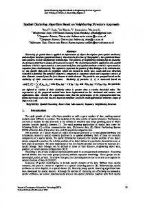
v) (A2, A5) = (A2, A6) = (A2, A10) = (A5, A8) = (A5, A9) = (A7, A8) = (A7, A9) = (A7, A11) = 0.5 a) As there are 5 similarity values greater or equal to cut-off so 5 graphs can be constructed from them. b) The members of these 5 graphs are: G1= {A5, A10}, G2 = {A9, A11}, G3= {A6, A12}, G4 = {A4, A5, A6, A9, A11} and G5 = {A2, A5, A6, A7, A8, A9, A10, A11} Explanation of Construction of Graphs: Let’s for example consider graph G4 shown in Figure 1. This connected weighted graph is constructed for similarity value 0.571428571, where the nodes are A4, A5, A6, A9 and A11. The edge weights between (A4, A9), (A4, A11), (A5, A6) and (A6, A9) are all 0.571428571. A4 A11

A9

A5

A6

Fig. 1. Graph G4 where the weight value of each edge is 0.571428571

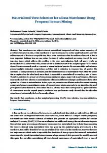
According to the algorithm, each graph is treated as a cluster. As 5 graphs are constructed so, 5 clusters (C1, C2, C3, C4 and C5) are formed from them. Hence after step 3, the set of materialized view C contains: C = {C1= (A5, A10), C2= (A9, A11), C3 = (A6, A12), C4= (A4, A5, A6, A9, A11), C5= (A2, A5, A6, A7, A8, A9, A10, A11)}. Step 4: The average similarity value (Ci) avg for each of the cluster centroid is calculated as: (C1)avg = 0.833333, (C2)avg =0.714285714, (C3)avg = 0.666667, (C4)avg = 0.5011905 and (C5) avg=0.411918 (Calculated according to equation 2) Explanation of Cluster Centroid Average Similarity Calculation: Let’s consider the calculation of cluster centroid average similarity for cluster C4. In fig. 1 only the edges which had weights 0.571428571 were drawn and a connected graph G4 was formed between the nodes A4, A5, A6, A9 and A11. The edges between (A4,A6),(A4,A5),(A5,A9),(A5,A11) ,(A6,A11) and (A9,A11) were not drawn and hence their weights were not considered in the graph construction method. Since each weight between the pair of nodes is the measure of association or similarity between the attributes. This fact is taken care of in this step. If complete graph with all the possible edges and their weights is drawn it would look like fig. 2. = =10.The similarity values beCluster C4 has 5 attributes (n=5), hence tween all pair of attributes inside cluster C4 are taken from section (4.Step 2) and rewritten below: (A4,A5)=0.375,(A4,A6)=0.428571429,(A4,A9)=0.571428571,(A4,A11)=0.571428571 ,(A5,A6)=0.571428571,(A5,A9)=0.5,(A5,A11)=0.333333,(A6,A9)=0.571428571,(A6,A11 )=0.375,(A9,A11)=0.714285714. The Total (∑ J A , A ) of the above values = 5.011905.

Materialized View Construction Based on Clustering Technique

A4

0.57428571

A11

0.428571429 0.375

0.333333 A5

0.375 A6

0.571428571

263

0.714285714 0.57428571

0.571428571 0.5

A9

Fig. 2. Modified graph G4 with all possible pair of nodes connected

The average (C4) avg = (5.011905 /10) = 0.5011905 (From equation 2). = Similarly for cluster C5 (n=8), (C5) avg can be calculated as (C5) avg = Total / (11.53371 / 28) =0.411918. [Refer to section (4.Step 2) for relevant data] We find that only for cluster C5 the cluster centroid average similarity is less than cut-off .So, C5 is rejected and the valid clusters are C1, C2, C3 and C4. Since every valid cluster is treated as a materialized view, so finally we have 4 materialized views created for the given database: View-1 (A5, A10), View-2 (A9, A11), View-3 (A6, A12) and View-4 (A4, A5, A6, A9, A11).

5

Performance of the Proposed Clustering Algorithm

K-means algorithm is most widely used clustering algorithm in different applications. The major drawbacks of the k-means clustering algorithm are: a) Number of desired clusters are predefined. However in this problem domain the numbers of clusters or materialized views can’t be fixed. b) There is a continuous shifting of cluster members to form the final valid clusters. This increases the time and computational complexity of the algorithm. In the proposed clustering algorithm the numbers of desired clusters is unknown at the beginning. There is no need to predefine the desired number of clusters. Secondly, the validation process of each cluster considers the cluster centroid similarity measure only and does not require any shifting between inter cluster members. After validation either a cluster is considered to be valid or is rejected. The valid clusters form the materialized views. In this way the proposed weighted graph based clustering algorithm outperforms k-means algorithm.

6

Conclusion and Future Work

The paper contributes to the formation of materialized views using clustering technique. The existing techniques worked with pair wise attribute association only and at no stage considered the association or similarity of multiple attributes at a time. This research gap is identified in this paper and a method is introduced which measures the similarity function of every attribute with all other attributes present and this

264

S. Roy, R. Ghosh, and S. Sen

knowledge guides the construction of materialized views in the forms of cluster. Further a method is introduced which measures the quality of the materialized views in terms of intra attribute association. Only those views which have a predefined intra attribute association are therefore considered as the final materialized views. This clustering based methodology may be further extended in distributed environment where the data servers are physically located in different geographical location. The proposed methodology need to be upgraded to consider access frequency of different queries at different sites, network bandwidth etc. to address the constraints of distributed systems. Apart from using the Jaccard Index the formation of distributed materialized views can also be done using other established similarity functions like Cosine Based Similarity and Tanimoto Coefficient. A comparative study of these methods and simulation in distributed environment would help to choose the appropriate methods for constructing materialized views.

References 1. Hu, Y., Zhai, W., Tian, Y., Gao, T.: Research and Application of Query Rewriting Based on Materialized Views. In: Qi, L. (ed.) ISIA 2010. CCIS, vol. 86, pp. 85–91. Springer, Heidelberg (2011) 2. Li, G., Wang, S., Liu, C., Ma, Q.: A modifying strategy of group query based on materialized view. In: IEEE 3rd International Conference on Advanced Computer Theory and Engineering (ICACTE), Chengdu, China, vol. 5, pp. 381–384 (2010) 3. Lee, M., Hammer, J.: Speeding up materialized view selection in data warehouses using a randomized algorithm. International Journal of Cooperative Information Systems 10(3), 327–353 (2001) 4. Vijay Kumar, T.V., Kumar, S.: Materialized View Selection Using Simulated Annealing. In: Srinivasa, S., Bhatnagar, V. (eds.) BDA 2012. LNCS, vol. 7678, pp. 168–179. Springer, Heidelberg (2012) 5. Derakhshan, R., Stantic, B., Korn, O., Dehne, F.: Parallel simulated annealing for materialized view selection in data warehousing environments. In: Bourgeois, A.G., Zheng, S.Q. (eds.) ICA3PP 2008. LNCS, vol. 5022, pp. 121–132. Springer, Heidelberg (2008) 6. Rashid, A.N.M.B., Islam, M.S., Hoque, A.S.M.L.: Dynamic materialized view selection approach for improving query performance. In: Das, V.V., Stephen, J., Chaba, Y. (eds.) CNC 2011. CCIS, vol. 142, pp. 202–211. Springer, Heidelberg (2011) 7. Phan, T., Wen, L.S.: Dynamic Materialization of Query Views for Data Warehouse Workloads. In: IEEE 24th International Conference on Data Engineering (ICDE), Cancun, Mexico, pp. 436–445 (2008) 8. Tang, N., Yu, X.J., Ozsu, T.M., Choi, B., Wong, K.-F.: Multiple Materialized View Selection for XPath Query Rewriting. In: IEEE 24th International Conference on Data Engineering (ICDE), Cancun, Mexico, pp. 873–882 (2008) 9. Liu, Z., Chen, Y.: Answering Keyword Queries on XML Using Materialized Views. In: IEEE 24th International Conference on Data Engineering (ICDE), Cancun, Mexico, pp. 1501–1503 (2008)

Materialized View Construction Based on Clustering Technique

265

10. Garnaud, E., Maabout, S., Mosbah, M.: Functional dependencies are helpful for partial materialization of data cubes. In: Garnaud, E., Maabout, S., Mosbah, M. (eds.) Springer Journal on Annals of Mathematics and Artificial Intelligence (August 14, 2013) 11. Li, H.-S., Huang, H.-K., Liu, S.: PMC: Select Materialized Cells in Data Cubes. In: Tjoa, A.M., Trujillo, J. (eds.) DaWaK 2005. LNCS, vol. 3589, pp. 168–178. Springer, Heidelberg (2005) 12. Sen, S., Dutta, A., Cortesi, A., Chaki, N.: A new scale for attribute dependency in large database systems. In: Cortesi, A., Chaki, N., Saeed, K., Wierzchoń, S. (eds.) CISIM 2012. LNCS, vol. 7564, pp. 266–277. Springer, Heidelberg (2012) 13. Sen, P.G.S., Chaki, N.: Materialized View Construction Using Linear Regression on Attributes. In: IEEE Proc. of the 3rd International Conference on Emerging Applications of Information Technology (EAIT ), Kolkata, India, pp. 214–219 (2012) 14. Schaeffer, S.E.: Survey on Graph Clustering. Elsevier Computer Science Review, 27–64 (2007), doi:10.1016/j.cosrev, 05.001