mining technique, more precisely the clustering of the query workload. ... Keywords: Materialized views, XML, Data warehouses, Clustering, Complex data. 1.
Materialized View Selection by Query Clustering in XML Data Warehouses Hadj Mahboubi, Kamel Aouiche and Jérôme Darmont ERIC – University of Lyon 2 5 avenue Pierre Mendès-France 69676 Bron Cedex, France {hmahboubi,kaouiche,jdarmont}@eric.univ-lyon2.fr
ABSTRACT XML data warehouses form an interesting basis for decision-support applications that exploit complex data. However, native XML database management systems currently bear limited performances and it is necessary to design strategies to optimize them. In this paper, we propose an automatic strategy for the selection of XML materialized views that exploit a data mining technique, more precisely the clustering of the query workload. To validate our strategy, we implemented an XML warehouse modeled along the XCube specifications. We executed a workload of XQuery decision-support queries on this warehouse, with and without using our strategy. Our experimental results demonstrate its efficiency, even when queries are complex. Keywords: Materialized views, XML, Data warehouses, Clustering, Complex data.
1. Introduction Decision support applications nowadays exploit heterogeneous data from various sources. Furthermore, the development of the Web and the proliferation of multimedia documents contributed to the analysis of so-called complex data [8]. For instance, analyzing medical data may lead to exploit jointly information under various forms: patient records (classical database), medical history (text), radiographies, echographies (multimedia documents), physician diagnoses (texts or audio recordings), etc. In this context, we have used XML in the process of integrating and warehousing complex data for analysis [7]. However, decision-support queries are generally complex because they involve several join and aggregation operations. In addition, native XML database management systems (DBMSs) present poor performances when the volume of data is very large and the queries are complex. Thus, it is crucial to design XML data warehouses that guarantee the best performance when accessing data. Indexing and view materialization are the most frequently used optimization techniques for this sake [12].
Materialized views are physical structures that improve data access time by precomputing intermediary query results. Then, end-user queries can be processed efficiently from the data stored within these views and do not need access the original data any more. Nevertheless, the use of materialized views requires additional storage space and induces some refreshing process overhead. So it is crucial to select only pertinent views. In the context of relational data warehouses, several studies have been proposed to resolve the materialized view selection problem [1, 3, 4, 10, 11, 13, 18, 22, 23, 24, 25, 27]. The views that are relevant to materialize are selected to minimize the processing time of a given workload. This optimization is achieved under maintenance cost or storage space constraints [16]. The existing studies differ in several points: 1. the way of determining candidate views; 2. the framework used to capture relationships between candidate views; 3. the use of mathematical cost models vs. calls to the query optimizer;
4. the selection of views in a relational or multidimensional context; 5. multiple or simple query optimization; 6. theoretical or technical solutions. The most recent approaches are workload-driven. They syntactically analyze the workload to enumerate the relevant candidate views [1]. By calling the query optimizer, they greedily build a configuration of the most pertinent views. A materialized view selection based on clustering has also been proposed [2]. This proposal exploits query clustering to determine a set of candidate views and cost models to choose pertinent views to materialize. To the best of our knowledge, no such view materialization approach exists in XML databases and XML data warehouses in particular. Hence, we propose in this paper an adaptation of the query clustering-based relational view selection approach [2] to the XML context. Our approach clusters XQuery queries (instead of SQL queries) and builds candidate XML views that can resolve multiple similar queries belonging to the same cluster. New XML-specific cost models are used to define the XML views that are pertinent to materialize. To validate our proposal, we implemented an XML data warehouse in a native XML DBMS. It is indeed interesting to check whether native XML DBMSs could someday be able to compete with XML-compatible, relational DBMSs. Then, we measured the execution time of a decision-support query workload with and without using our strategy. Our experimental results show that the use of our strategy greatly improves query performance. The remainder of this paper is organized as follows. We first present the context of this study in Section 2. Then we detail our materialized view selection strategy in Section 3. In order to validate our strategy, we present some experimental results in Section 4. Finally, we conclude and outline some research perspectives in Section 5.
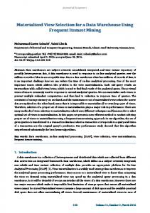
2. Study context 2.1 XML data warehouse specification Several studies have been proposed for designing and building XML data warehouses. For instance, Pokorny modeled a star schema in XML by defining dimension hierarchies as a set of logically connected collections of XML data, and facts as XML data elements [20, 21]. Park et al. also proposed an XML multidimensional model in which each fact is described by a single XML document and dimension data are grouped into a repository of XML documents [19]. Finally, Hummer et al. designed XCube, a family of templates allowing the description of a multidimensional structure, dimension and fact data for integrating several data warehouses into a virtual or federated data warehouse [14]. The federated templates are not directly related to XML warehousing, but they can be used to represent XML star schemas. XCube is organized as a set of modules or formats: XCube Schema, XCube Dimensions and XCube Facts, which respectively formalize the schema, the dimensions and the facts according to a star schema. These studies use XML documents to manage or represent the facts and dimensions of an XML data warehouse. They actually help logically modeling a data warehouse. This allows the native storage of documents and their easy interrogation based on XML languages. In this paper, we selected the XCube specification to model a reference XML data warehouse and apply our strategy. Indeed, in XCube, the authors proposed a simple structure for representing facts and dimensions in a star schema. They use one XML document to represent dimensions and one XML document to represent facts. In addition, they use another XML document representing warehouse metadata. The other proposals do not use XML documents for representing warehouse
schema. However, we need these metadata to compute our cost models. Thus, our data warehouse is composed of the following XML documents: • Schema.xml specifies the data warehouse metadata; • Dimensions.xml defines all the dimensions characterized by their attributes and values; • Facts.xml specifies the facts, i.e., the identifiers of dimensions and the description of measures.
Figure 1. XCube warehouse specification 2.2 XML data warehouse interrogation We selected the XQuery language [5] to formulate our decision-support queries because, unlike simpler languages such as XPath, it allows complex queries, including join queries over multiple XML documents, to be expressed with the FLWOR syntax. However, in our implementation, we had to extend FLWOR expressions with explicit Group by clauses to be able to formulate the decisionsupport queries we needed. Thus, we added the functions Group by (attribute list) and Aggregation (aggregation operations, measure list) to the XQuery syntax. Figure 2 provides an example of decision-support query with a multiple Group by clause.
Figure 2. Decision-support XQuery example
3. XML materialized selection strategy
view
The architecture of our materialized view selection strategy is depicted in Figure 3. We assume that we have a workload composed of representative queries for which we want to select a configuration of materialized views in order to reduce their execution time. The first step is to build, from the workload, a clustering context. Then we define similarity and dissimilarity measures that help clustering together similar queries. For each cluster, we build a set of candidate views. The last step exploits cost models that evaluate the cost of accessing data using views and the cost of their storage to build a final materialized view configuration.
Figure 3. Materialized view selection strategy
In practice, it is hard to search all the syntactically relevant views (candidate views) because the search space is very large [1]. To reduce the size of this space, we propose to cluster the queries. Hence, we group in a same cluster all the queries that are similar. Similar queries are the one having a close binary representation in the query-attribute matrix. Two similar queries can be resolved by using only one materialized view. We define similarity and dissimilarity measures that ensure that queries within a same cluster are strongly related to each others whereas queries from different clusters are significantly different. 3.2.1 Similarity and dissimilarity measures A query is described by the attributes extracted in the query analysis phase. We thus describe a query qi by a vector qi = {q1i , q 2i ,..., q pi }, where p is the
Figure 4. Workload snapshot 3.1 Query workload analysis The workload that we consider is a set of selection, join and aggregation queries. Figure 4 gives a snapshot of this workload. The first step consists in extracting from the workload the representative attributes for each query. We mean by representative attributes those are present in Where (selection predicate attributes) and Group by clauses. We store the relationships between the query workload and the extracted attributes in a “query-attribute” matrix. The matrix lines are the queries and the columns are the extracted attributes. A query qi is then seen as a line in the matrix that is composed of cells corresponding to representative attributes. The general term qij of this matrix is set to one if extracted attribute ai is present in query qi , and to zero otherwise. This matrix represents our clustering context. Table 1 shows the query-attribute matrix that is built from the workload snapshot from Figure 4. 3.2 Building configuration
the
candidate
view
number of attributes in the matrix. This description allows query comparison. We define similarity (respectively, dissimilarity) between two queries qi and
qj
regarding attribute a k (k = 1.. p ) in
Formula 1 (respectively, Formula 2). ⎧1 if q ki = q kj = 1
δ sim (q ki , q kj ) = ⎨
⎩0 otherwise ⎪⎧1 if q ki = q kj δ dissim (q ki , q kj ) = ⎨ ⎪⎩0 if q ki ≠ q kj
(1)
(2)
Two queries qi and q j are similar regarding
attribute
ak
if
and
only
if q ki = q kj = 1 , i.e., a k is present in both queries. They are dissimilar if and only if q ki ≠ q kj , i.e., one of the two queries does not contain attribute a k . These measures can be extended to a set A composed of p attributes such that we get the degree of global similarity and dissimilarity between two queries. We thus define the similarity (respectively, dissimilarity) between two queries qi and
q j according to all the matrix attributes a k in Formula 3 (respectively, Formula 4).
p
sim(qi , q j ) = ∑ δ sim (q ki , qlj )
(3)
j =1
0 ≤ sim(qi , q j ) ≤ p p
dissim(qi , q j ) = ∑ δ dissim (q ki , qlj )
(4)
j =1
0 ≤ dissim(qi , q j ) ≤ p
Thus,
the
closer
sim(qi , q j )
(respectively, dissim(qi , q j ) ) is to p , the more qi and q j are considered similar (respectively, dissimilar). We also define similarity (respectively, dissimilarity) measures between two query sets and within a query set. These measures are defined by Formulas 5, 6, 7 and 8. sim(C a , C b ) =
∑δ
sim qk ∈C a , ql ∈Cb
(q k , ql )
(5)
0 ≤ sim(C a , C b ) ≤ card (C a ) × card (C a ) × p dissim (C a , C b ) = ∑ δ dissim ( q k , ql ) (6) qk ∈C a , ql ∈Cb
0 ≤ dissim (C a , C b ) ≤ card (C a ) × card (C a ) × p
sim(C a ) =
∑δ
sim qk ∈Ca , ql ∈Cb , k