Randall T. Anderson2 e-mail:
[email protected]
Perry Y. Li
Mathematical Modeling of a Two Spool Flow Control Servovalve Using a Pressure Control Pilot1
e-mail:
[email protected] Department of Mechanical Engineering, University of Minnesota, 111 Church St. SE, Minneapolis, MN 55455
I
A nonlinear dynamic model for an unconventional, commercially available electrohydraulic flow control servovalve is presented. The two stage valve differs from the conventional servovalve design in that: it uses a pressure control pilot stage; the boost stage uses two spools, instead of a single spool, to meter flow into and out of the valve separately; and it does not require a feedback wire and ball. Consequently, the valve is significantly less expensive. The proposed model captures the nonlinear and dynamic effects. The model has been coded in Matlab/Simulink and experimentally validated. 关DOI: 10.1115/1.1485287兴
Introduction
The vast majority of flow control servovalves in existence employ a double flapper nozzle pilot stage and a single spool boost stage. A stiff feedback spring is generally used to provide feedback from the boost stage to the pilot. These types of servovalves tend to be difficult to manufacture and expensive. A less conventional, less costly type of flow control servovalve 关1,2兴 utilizes a two-spool boost stage and a flapper nozzle pressure control pilot. Because a feedback wire between the nozzle flapper pilot and the boost stage is not needed, assembly is simplified. The two spools in the boost stage are spring loaded and meter flow into and out of the valve separately. The main advantages of the two-spool/ pressure control pilot design are: 共1兲 ease of manufacturing; 共2兲 lower costs; 共3兲 higher degree of adjustment; and 共4兲 greater safety. Because flow into and out of the valve are metered separately using separate spools, the required machining accuracy of the land lengths and of the metering edges are significantly reduced. The shorter bore lengths enable better machining of the metering edges. Electrical displacement transducers are not necessary. The main cost advantage stems from the fact that the two porting edges can be independently machined, so that each bore only has one critical axial dimension, in contrast to a conventional design in which three critical dimensions are interrelated to each other. In addition, the two spool design allows the use of modular components, the boost stage housing needs machining only from two sides. The valve can also be easily adjusted for different applications since each spool can be independently positioned. The two-spool design is also potentially safer because unless both spools are jammed open, flow can be shutoff by either spool. Servovalves that utilize the two-spool/pressure control pilot design have a better cost/performance ratio, although they do have lower performance 共open loop bandwidth兲 than their conventional counterparts. The objective of this paper is to present a complete and validated nonlinear dynamic model for this unconventional two-stage two-spool valve, with similar details as in the models for conventional servovalves, which are readily available 共e.g. 关3,4兴兲. This is needed in order to predict system performance and stability, and to design control systems in high performance applications. A mathematical model relating the various physical parameters to performance can also be used to predict and improve the performance in 1 An abridged version of this paper was first presented at the ASME IMECE 2000 in Orlando, FL. 2 R. Anderson is currently at Eaton Corporation, Eden Prairie, MN. Contributed by the Dynamic Systems and Control Division for publication in the JOURNAL OF DYNAMIC SYSTEMS, MEASUREMENT, AND CONTROL. Manuscript received by the Dynamic Systems and Control Division February 2001. Associate Editor: N. Manring.
420 Õ Vol. 124, SEPTEMBER 2002
the physical design of the valves. Anderson 共who holds the patent on the design兲 presented simplified linear models in 关5兴. A complete derivation of the model, such as the loading effect of each subsystems on each other is, however, not presented. Although the importance of the nonlinearities associated with the valves is mentioned, they are not included in these simplified models. In this paper, an experimentally validated physical model of the valve is presented. The model takes into account nonlinear effects such as flow forces, nonlinear magnetic effects, and chamber fluid compressibility. The model is capable of predicting the dynamic output flow rate when time trajectories of the electrical current input and of the work port pressures are given. The model prediction compares favorably with experimental data. In a companion paper 关6兴, the model is used to provide a basis for the analysis for performance limitation and for the dynamic redesign to improve performance. It will be demonstrated how the structure of the interconnection of the subsystems limits the dynamic performance. After this paper was first submitted, the authors were made aware of the earlier modeling efforts by Akers and co-workers on valves related to the one investigated here. They presented a model for a two-stage, two-spool pressure control valve in 关7兴. A model for the two-spool two-stage flow control valve similar to the one in this paper was presented at the ASME Winter Annual Meeting in 关8兴. Differences between the two models will be discussed after the presentation of the model. The rest of the paper is organized as follows. The basic operation of the valve is given in Section II. The models for each subsystem are then developed. The models for the pilot and the boost stages are presented in Sections III and IV, respectively, the chamber pressure dynamics are given in Section V, and the output flow equations are given in Section VI. In Section VII, simulation issues are discussed. Simulation and experimental results are shown in Section VIII. Conclusions are given in Section IX. A table of nomenclature appears at the end of the paper.
II
Operation of the Two-Spool Valve
A schematic of the flow control servovalve using a two-spool boost stage, and pressure control pilot design is shown in Fig. 1. It consists of two distinct stages—a pilot and a boost stage, separated by a simple transition plate and connected via two pressure chambers. The pilot stage is a pressure control pilot 关9兴, which uses a double nozzle flapper design. The boost stage of the valve consists of two separate spring centered spools which meter flow into and out of the valve separately. Roughly speaking, the pressure control pilot stage generates a differential pilot pressure 共i.e., the pressure difference between the two pressure chambers兲 proportional to the electrical current input
Copyright © 2002 by ASME
Transactions of the ASME
Fig. 1 Schematic of the two spool flow control valve using a pressure control pilot
to the electromagnetic torque motor. The differential pilot pressure in the chambers acts on the two ends of both spools. Since the spools are spring centered, the steady-state displacements of the spools are roughly proportional to the differential pilot pressure and inversely proportional to the total stiffness 共which would include effects of steady-state flow forces兲. Flows into and out of the valve are metered by the displacements of the spools. Notice that a feedback wire between the boost stage and the pilot stage is not used in this design. The interconnection between the subsystems of the valve is shown in Fig. 2. A more detailed discussion of the operation of the valve follows. Suppose that the electrical current is the input to the coil of the torque motor at the top part of the valve in Fig. 1. The current in the coil, together with the magnetic armature, generates a torque, which in turn rotates the armature and flapper in the counter-clockwise motion about the pivot point 共where the armature and the flapper intersect兲. Note that in Fig. 1, bold arrows correspond to the direction of fluid flow. As the flapper is displaced to the right 共left兲, the nozzle opening on the right 共left兲 decreases and the opening on the left 共right兲 increases. This in turn raises P 2 and lowers P 1 共or vice versa兲 in the pressure chambers. The differential pressure P 2 ⫺ P 1 , therefore, has the effect of restoring the flapper to its neutral position. As will be seen later, the torque provided by the torque motor increases with the flapper Journal of Dynamic Systems, Measurement, and Control
Fig. 2 Signal flow and subsystem interconnection diagram of the valve
SEPTEMBER 2002, Vol. 124 Õ 421
displacement. Thus, it presents itself as a negative stiffness. By magnetizing/demagnetizing the permanent magnet in the torque motor, this negative stiffness is used to cancel out the mechanical stiffness of the pivot 关5兴. When this is true, the torque generated in the torque motor will be balanced predominantly by the differential pressure P 2 ⫺ P 1 . Consequently, in the steady state, the differential pressure will be roughly proportional to the input current. The pilot pressures, P 1 and P 2 , act on the two ends of each spool. A positive 共negative兲 differential pressure P 2 ⫺ P 1 causes both spools to move in the upward 共downward兲 direction. As spools A and B move upward 共downward兲, hydraulic oil is ported from the supply to port B 共A兲 on one side, and from port A 共B兲 into the tank on the other, creating flows Q b and Q a , respectively. As the spools displace, flows Q 1 to and Q 2 from the pilot stage are also created. The regulation of the spool displacements 共hence the flow rate兲 is achieved in two ways. Primarily, displacements of the spools are resisted by the compression of the springs. Thus, in the steady state, the displacement of each spool would be proportional to the differential pilot pressure and inversely proportional to the spring stiffness. Secondarily, the displaced fluid volume above and below the spools also tend to reduce the differential pressure. Therefore, the upward 共downward兲 spool displacement and velocity tend to decrease P 2 ⫺ P 1 . These effects in turn affect the flapper displacement and the differential pilot pressure. If the system is stable, the spool will reach an equilibrium displacement.
Fig. 3 Free body diagram of the armature-flapper
␣ 3 ⫽2 r-plateA a A b NM o ␣ 4 ⫽ r-plateA a A b G g M 2o ⫹ r-siliconA a A g G b M 2o ⫹2 r-plateA b A g G a M 2o
 1 ⫽ r-plateA a A b G 2g ⫹ r-siliconA a A g G b G g ⫹2 r-plateA b A g G a G g
III
 2 ⫽ r-plateA a A b .
Pilot Stage Dynamics
We now derive the physical model for each subsystem, beginning with the pilot stage. The free body diagram of the armatureflapper assembly is shown in Fig. 3. Note that O is the pivot point supported on a torsional beam spring, and is the anti-clockwise angular displacement of the armature-flapper, which is assumed to be small. The armature-flapper is subjected to the magnetic force, F g , generated at the top air gap, the trim spring force, F k , at the top end of the armature, the damping moment B f ˙ on the armature 共created as the armature moves in the silicon oil that fills the area above the flapper兲, the moment K p due to the pivot stiffness, and the flow and pressure forces due to the nozzle, F f . L k , L g , and L f are the moment arms about the pivot O for the trim spring force, the magnetic force F g and the nozzle flow force F f , respectively. The magnetic force, F g , is found by analyzing the magnetic circuit shown in Fig. 4. R a is the reluctance due to the lower air gap between the magnetic plate and the armature, while R b is the reluctance between the polepieces and the magnetic plate. R 1 and R 2 correspond to the reluctances at the two top air gaps between the polepieces and the armature. They are functions of the linear armature displacement, x g ⫽L g . Referring to Fig. 4, the magnetic force in the air gap is given by 关3兴: F g ⫽4.42⫻10⫺8
再
冎
21 ⫺ 22 lb, 0A g
Next, the moment due to the trim spring is considered. Because there are two trim springs with spring constant K k , the total counterclockwise moment due to the trim spring is: ⫺L k F k ⫽⫺2K k x k ⫽⫺ 共 2K k L k 兲 .
(3)
Nozzle forces on the flapper are given by 关3兴: F f ⫽ 共 P 2 ⫺ P 1 兲 A n ⫹4 C d2 f 关共 x f o ⫺x f 兲 2 P 2 ⫺ 共 x f o ⫹x f 兲 2 P 1 兴 (4) where the first term corresponds to the static pressure force, and the second term corresponds to the flow forces at the nozzle, and x f ⫽L f is the displacement of the flapper. The pivot spring of the armature-flapper is a rectangular beam, therefore, the pivot stiffness 共in-lb/rad兲 is 关10兴: K p ⫽2
冋
冉
h t w t3 16 w t4 wt ⫺3.36 1⫺ 16 3 ht 12h t4
冊册
G Lf
(5)
which is valid for w t ⬍h t . Summing moment about the pivot, we obtain:
(1)
where 1 ⫽ x ⫹ y , and 2 ⫽ x ⫹ z . It can then be shown that: F g⫽ ␣ 0
␣ 1 •i⫹ ␣ 2 • 共 i 2 x g 兲 ⫹ ␣ 3 • 共 ix 2g 兲 ⫹ ␣ 4 •x g 共  1 ⫺  2 x 2g 兲 2
(2)
where 2 ␣ 0 ⫽4.42x10⫺8 o r-silicon r-plateA a A b A g
␣ 1 ⫽2 r-plateG g NM o 共 2A b G a A g ⫹A a A b G g 兲 ⫹2 r-siliconA g G g A a G b NM o
␣ 2 ⫽4 r-plateA a A b G g N 2 422 Õ Vol. 124, SEPTEMBER 2002
Fig. 4 Armature magnetic circuit. R 1 , R 2 represent the variable air-gaps; R a , R b represent the fixed air-gaps. N " i and M 0 are the MMF’s due to the input current and the permanent magnet, respectively.
Transactions of the ASME
J ¨ ⫽F g L g ⫺F k L k ⫺F f L f ⫺K p ⫺B f ˙
(6)
where J is the moment of inertia of the armature-flapper. Using the relationships ⫽x f /L f ⫽x g /L g , 共6兲 can be written in terms of x f and x˙ f . This way, we obtain a second-order model for the pilot stage in the form of x¨ f ⫽ f pilot共 x f ,x˙ f ,i, P 1 , P 2 兲
(7)
where x f and x˙ f are states, and i, P 1 and P 2 are the inputs.
IV
Boost Stage Dynamics
The model for the boost stage is developed next. We need to derive the dynamic equations that describe the two spools. We will analyze spool A in Fig. 5 in detail. The equations for spool B can be similarly derived. We assume the spools are designed to be critically centered. In Fig. 5, the spool is subjected to the differential pilot pressure, a force due to the centering spring, viscous friction and flow forces. Equating forces on the spool yields the following: M s x¨ a ⫽ 共 P 2 ⫺ P 1 兲 A s ⫺2K s x a ⫺F V ⫺F F,A
(8)
where RHS are forces due to the differential pressure, 2K s x s is the force due to the two centering springs of stiffness K s , F F,A corresponds to the flow forces, and F V is the viscous damping force. Assuming a perfectly centered spool in a bore 关3兴, the viscous damping force is: F V⫽
D sL s ˙x a . Cr
(9)
The fluid flow forces F F that the spool encounters are sometimes called Bernoulli forces which arise due to the dynamics of the fluid flow. There are two types of flow forces: steady-state flow forces and transient flow forces. Steady-state flow forces are due to the angle of the vena contracta as the fluid is metered into or out of the valve. They depend on the flow rate and hence the spool displacement. Transient flow forces, on the other hand, are the reactive forces associated with the acceleration of the fluid in the spool chamber. Thus, they are dependent on the rate of change of flow and the spool velocity. The signs of the steady-state and transient components depend on the spool displacements, velocities, and on whether the spool is metering flow into or out of the valve. Following 关3兴, the fluid flow forces on spool A are given by:
F F,A ⫽
冦
C d j C w 共 P a ⫺ P T 兲 cos共 j 兲 •x a
⫹L p C d j w 冑2 共 P sb ⫺ P a 兲 •x˙ a
x a ⭓0
⫺L p C d j w 冑2 共 P sb ⫺ P a 兲 •x˙ a
x a ⬍0.
C d j C w 共 P sb ⫺ P a 兲 cos共 j 兲 •x a
(10)
where the first term corresponds to the steady-state flow force, and the second term corresponds to the transient flow force. In Eq. 共10兲, the effect of clearance can be taken in account by replacing x a by sign(x a ) 冑x 2a ⫹C r2 in the first term. Notice that regardless of the sign of x a , the steady-state flow force is always restoring and acts like a spring to close the valve. On the other hand, the transient flow force is proportional to the spool velocity. It acts like a positive stabilizing damping when x a ⭓0 共when flow is being metered out of the valve兲. However, when x a ⬍0 when 共flow is being metered into the valve兲, it acts like a negative, unstable damping. Transient flow forces therefore can be a source of valve instability. A recent investigation into the benefits of exploiting the instability induced by transient flow force is given in 关11兴. In Eq. 共10兲, L p , is the damping length, which is the length of the fluid column that undergoes acceleration. The transient flow force is therefore proportional to the damping length. For the valve being considered, L p depends on the spool displacement: L p ⫽L po ⫹
1 兩x 兩 2 a
where L po is the damping length when the spool displacement is zero. Since the stroke lengths of the main spools are about 20% of L po , the transient flow force can be underestimated by as much as 10% if L p is assumed to be L po . In Eq. 共10兲, j is the fluid jet angle of the vena contracta. It is a nonlinear function of x a /C r 关3兴. j varies from 69 deg at large spool displacements to 21 deg at small orifice openings. These differences can cause large deviations in the steady-state flow force term (cos(21deg)/cos(69deg)⫽2.6). Thus, using only a constant jet angle throughout the range of spool displacements may not be adequate. To account for this variation, the variation in jet angle when the orifice opening varies is explicitly modeled using a high order polynomial to represent the nonlinear dependence of j on x s /C r as shown in 关3兴. The dynamics for spool B can be similarly obtained: M s x¨ b ⫽ 共 P 2 ⫺ P 1 兲 A s ⫺2K s x b ⫺
D sL s ˙x b ⫺F F,B , Cr
(11)
where the downward flow forces for spool B are:
F F,B ⫽
冦
C d j C w 共 P sb ⫺ P b 兲 cos共 j 兲 •x b
⫺L p C d j w 冑2 共 P sb ⫺ P b 兲 •x˙ b ,
x b ⭓0
⫹L p C d j w 冑2 共 P b ⫺ P T 兲 •x˙ b ,
x b ⬍0.
C d j C w 共 P b ⫺ P T 兲 cos共 j 兲 •x b
(12)
Substituting Eqs. 共9兲–共10兲 into 共8兲, and 共12兲 into 共11兲, the dynamics of the two spools are described by two sets of second order dynamic systems, of the form:
Fig. 5 Free body diagram for spool A
Journal of Dynamic Systems, Measurement, and Control
x¨ a ⫽ f sp1 共 x a ,x˙ a , P 1 ⫺ P 2 , P a 兲
(13)
x¨ b ⫽ f sp2 共 x b ,x˙ b , P 1 ⫺ P 2 , P b 兲
(14)
where the spool displacements and velocities x a and x˙ a , x b and x˙ b are the states, and the differential chamber pressure P 1 ⫺ P 2 and work port pressures P a , P b are the inputs. Notice that the work port pressures affect the spool dynamics only via the flow forces in Eqs. 共10兲 and 共12兲. SEPTEMBER 2002, Vol. 124 Õ 423
V
Chamber Pressure Dynamics
VI
The pilot pressures P 1 and P 2 are needed as inputs to both the pilot Eq. 共7兲, and the boost stage Eqs. 共13兲–共14兲 dynamics. These are determined by the compressibility of the fluid in the chambers between the pilot stage and the boost stage. The chamber pressures P 1 and P 2 are determined by the basic hydraulic compressibility equations: P˙ 1 ⫽ 
Q 1 ⫺V˙ 1 V 1共 t 兲
(15)
P˙ 2 ⫽ 
Q 2 ⫺V˙ 2 , V 2共 t 兲
(16)
where V 1 (t) and V 2 (t) are the volumes of the chambers between the top of the spools and the left flapper face, and between the bottoms of the spools and the right flapper face, respectively, Q 1 and Q 2 are the total flows into the chambers. Recall that an upward spool displacement is defined to be positive. The chamber volumes and their derivatives are therefore given by: V 1 ⫽V 1o ⫺A s x a ⫺A s x b ,
(17)
V 2 ⫽V 2o ⫹A s x a ⫹A s x b
(18)
V˙ 1 ⫽⫺A s x˙ a ⫺A s x˙ b ,
(19)
V˙ 2 ⫽A s x˙ a ⫹A s x˙ b
(20)
where V 1o and V 2o are the fluid volumes in all the lines and chambers between spool ends and the flapper when the spools are centered (x a ⫽x b ⫽0). The flows Q 1 and Q 2 into the chambers comprise of the flow from the pilot supply orifice, leakage past the nozzle, and leakage past the spools. Combining these three contributions, we get: Q 1 ⫽C d0 A 0
冑
2 共 P ⫺ P 1 兲 ⫺C d f D n 共 x f 0 ⫹x f 兲 sp
冑
2 P 1
D b C r3 P 1 D b C r3 共 P sb ⫺ P 1 兲 ⫺ ⫹ 12 共 L l0 ⫹x a 兲 12 共 L l0 ⫹x b 兲 Q 2 ⫽C d0 A 0 ⫹
冑
2 共 P ⫺ P 2 兲 ⫺C d f D n 共 x f 0 ⫺x f 兲 sp
D b C r3 共 P sb ⫺ P 2 兲 D b C r3 P 2 ⫺ 12 共 L l0 ⫺x a 兲 12 共 L l0 ⫺x b 兲
Flow Equations
As the spools in the boost stage move, flow is either metered into or out of the valve through the orifice. In addition to the orifice flow, the total flow at the work ports is also contributed by leakage flows through the spool-bore clearance 共see Fig. 6兲. Leakage is again modeled by laminar flow in an annulus between an annular shaft and a concentric cylinder. For spool A in Fig. 6, when the spool displacement is positive 共upwards兲, the flow paths 1, 5, 6 are active; and for negative displacements, flow paths 3, 5, 6 are active. Therefore, the flow into the valve from the work port A is:
Q a⫽
冑
2 P 2
冑
2 共 P a ⫺ P T 兲 D b C r3 共 P a ⫺ P T 兲 ⫹ 12 共 L li ⫺x a 兲 ⫺
C d wx a
D b C r3 共 P sb ⫺ P a 兲 12 共 L li ⫹x a 兲
x a ⭓0
冑
2 共 P sb ⫺ P a 兲 D b C r3 共 P a ⫺ P T 兲 ⫹ 12 共 L li ⫺x a 兲 ⫺
D b C r3 共 P sb ⫺ P a 兲 12 共 L li ⫹x a 兲
x a ⬍0. (25)
The first term in each of the two cases correspond to the orifice flow, and the other terms correspond to the leakage. Notice that when x a ⬍0, the orifice flow term Q a is negative indicating fluid flows out of the valve. For spool B and for positive spool displacement, the flow paths 2, 7, 8 are active in Fig. 6. When the spool displacement is negative, flow paths 4, 7, 8 are active. Hence,
Q b⫽ (21)
¦
C d wx a
¦
C d wx b
冑
2 共 P sb ⫺ P b 兲 D b C r3 共 P sb ⫺ P b 兲 ⫹ 12 共 L li ⫺x b 兲 ⫺
C d wx b
冑
D b C r3 共 P b ⫺ P T 兲 12 共 L li ⫹x b 兲
x b ⭓0
2 共 P b ⫺ P T 兲 D b C r3 共 P sb ⫺ P b 兲 ⫹ 12 共 L li ⫺x b 兲 ⫺
D b C r3 共 P b ⫺ P T 兲 12 共 L li ⫹x b 兲
x b ⬍0. (26)
(22)
where the leakages are modeled to be laminar flows in an annulus between a annular shaft and a concentric cylinder 关3兴. From 共15兲 and 共21兲 共and 共16兲 and 共22兲兲, one can see that the chamber pressure dynamics are stable since increase in P i decreases flow Q i , which in term decreases P˙ i . Substituting Eqs. 共17兲–共22兲 into Eq. 共15兲–共16兲, we have P˙ 1 ⫽ f cham1 共 P 1 ,x f ,x a ,x b ,x˙ a ,x˙ b 兲
(23)
P˙ 2 ⫽ f cham2 共 P 2 ,x f ,x a ,x b ,x˙ a ,x˙ b 兲
(24)
where P 1 and P 2 are the respective states, and the flapper displacements and the spool displacements and velocities are the inputs. At this point, all of the necessary differential equations have been developed to describe the pilot stage, spool A, spool B, and the chamber pressures, P 1 and P 2 . There are, in total, eight state variables. Next, we describe how the output flows at the work ports are related to the states of the valve. 424 Õ Vol. 124, SEPTEMBER 2002
Fig. 6 Flow paths when spools are displaced from null positions
Transactions of the ASME
Notice that Eqs. 共25兲–共26兲 have been derived with the assumption that 0⫽ P T ⭐ P a , P b ⭐ P sb . The signs of the terms in 共25兲–共26兲 must be suitably modified if this assumption is violated. Equations 共25兲–共26兲 define the flow that enters the valve through work port A, and the flow that leaves the valve through work port B. Beyond the work ports, there are other losses, including channels in the body, lines, fittings, etc. These should also be taken into consideration when calculating the flow in a complete system.
VII
MatlabÕSimulink Model
The dynamic models for the pilot stage, Eq. 共7兲, boost stage Eqs. 共13兲–共14兲, and the chamber pressure dynamics Eqs. 共23兲– 共24兲 can be connected to each other, and to a hydraulic device, such as in Fig. 2, into a simulation model. The combined model will be capable of predicting the flows Q a , Q b into and out of the work ports, given the input of the time trajectories of the electrical input current, i, and the two work port pressures P a , P b . In order to simplify the testing procedure, it will be convenient to assume that Q a ⫽Q b , i.e., the valve is connected to volume conserving devices 共such as a double ended cylinder or a hydraulic motor兲. This allows us to specify only the load-pressure, P L ª P b ⫺ P a , instead of specifying P a and P b independently. To this end, we calculate P a and P b given P L . Equating the output flows in Eq. 共25兲–共26兲, and neglecting the leakage flows, we obtain for usual combinations of x a , and x b : If x a , x b ⭓0 P a⫽
x 2b 共 P sb ⫺ P L 兲 x 2a ⫹x 2b
,
P b⫽
,
P b⫽
x 2b P sb ⫹x 2a P L x 2a ⫹x 2b
(27)
If x a , x b ⬍0 P a⫽
x 2a P sb ⫺x 2b P L x 2a ⫹x 2b
x 2a 共 P sb ⫹ P L 兲 x 2a ⫹x 2b
.
(28)
When x a and x b are of different signs 共which generally does not occur兲, it would be necessary to assume that P a or P b is either above P sb or below P T . In this situation, the simplifying assumption that Q a ⫽Q b is probably not valid. With the simplification that Q a ⫽Q b , the Matlab/Simulink model with the subsystem inter-connections and the input and output connections is shown in Fig. 7. The model of each of the
subsystems 共pilot, boost, pressure chambers兲 and the output flow equations, have been developed in a complete manner without resorting to empirical simplifications. All the parameters of the models, except for the pilot damping coefficient B f , are estimated from the component characteristics and the physical valve design. B f is determined to match the experimental results. The subsystems were coded using the S-Function facility instead of completely graphically because of the model complexities. Notice that the S-Function for the pilot stage receives as inputs, the input current i and the pilot pressures P 1 , P 2 on the flapper. Each of the spool S-Functions also receive the same pilot pressures P 1 , and P 2 , work port pressure drop P L and boost stage supply pressure P sb . The work port pressures P a and P b are calculated according to 共27兲–共28兲 in the subsystems given the load pressure P L and the spool displacements x a , x b . Notice in Fig. 7 that the operation of the two-spool/pressure control pilot valve utilizes two feedback loops in its design. The principal feedback loop consists of the pilot stage, and the pressure dynamics. This feedback loop controls the differential pilot pressure. The secondary loop involves the boost stage and the pressure dynamics. As mentioned in the Introduction, a similar model for the twostage two-spool flow control valve was presented in 关8兴. There are some differences between the present model and the one in 关8兴. For example, the nonlinearity in the coefficients 共L p and j 兲 for both the steady state and transient flow forces are treated in Eq. 共10兲 whereas in 关8兴 are treated as constants. More importantly, in this paper, we do not assume an apparent flapper pivot stiffness. Rather, the flapper dynamics Eq. 共6兲 are computed based on first principles, accounting for the magnetics, mechanical stiffnesses, and pressure forces. In 关8兴, however, the negative stiffness due to the magnetics in the torque motor is assumed to cancel out the flapper’s mechanical stiffness. As is shown in 关6兴, the value of the apparent mechanical stiffness can be important in the determination of the dominant valve dynamics.
VIII
Simulation and Experimental Results
To validate the model, the Simulink model is exercised and the results compared with experimental results under similar conditions. The experimental setup 共Fig. 8兲 consists of the two-spool flow control valve connected to a flow motor via a set of butterfly valves. The speed of the flow motor is measured via a magnetic pulse pick up and provides the surrogate flow measurement. The current input to the valve can be adjusted continuously using a computer. The butterfly valves can be adjusted offline to simulate different load pressures P L . The pilot pressures, P 1 and P 2 , as well as the work port pressures P a and P b are measured. A Steady-State Response. The steady-state flow Q versus current i 共at no load兲 and Q versus load pressure P L 共at various current i’s兲 plots are used to assess the steady-state response 共Fig. 9兲. For the Q versus i plot, the current was varied between ⫾40
Fig. 7 Simulink block diagram
Journal of Dynamic Systems, Measurement, and Control
Fig. 8 Schematic of the experimental setup
SEPTEMBER 2002, Vol. 124 Õ 425
Fig. 9 Steady-state response. Top: flow Q a versus input current; bottom: flow Q a versus load pressures P L at various currents i .
mA 共⫾100%兲 sinusoidally at 0.25 Hz. From Fig. 9, we see that the simulation and experiments show excellent match. Despite a slight hysteresis, the relationship between input current i and noload flow Q is quite linear. To obtain the Q versus P L plot, the load pressure was varied between 0 psi to 3075 psi ( P sb ) slowly. Figure 9 shows the familiar square root power relationship, as expected from Eqs. 共25兲–共26兲. Multiple experiments are included in Fig. 9 and the resolution of the flow measurement during this experiment was set at only 0.1 gpm. So the range and the discrete nature of the multiple dots corresponds to the measurement uncertainty and the limited resolution. Notice that the simulation results fall within this range. B Dynamic Responses. To evaluate the time response of the valve, various step current inputs at near zero load pressure drop were applied to the model and to the experimental setup. Because of the limitation of the current driver in the experimental setup, the actual current steps were not ideal and there were slight overshoots and finite rise times about 共8 ms兲. The nonideal ‘‘step’’ current inputs were measured during the experiments and were also used as the input for the simulations. The near step responses are shown in Fig. 10. Notice that the experimental and simulated responses are very similar; both showing 64% rise-times of approximately 20 to 30 ms. Notice from Fig. 10 that the experimental data has a time delay of about 4 ms relative to the simulation. This may be an artifact of our data acquisition system or due to the flow motor used for flow measurement having a finite inertia. Also, the hydraulic lines used in the experiments are quite flexible. These can also cause some overshoot. This is confirmed by a later test conducted with the valve mounted directly on the flow motor in which the large overshoot was not present 共not shown兲. Taking into account the risetime of the input step, and the measurement delay, the actual 共64%兲 risetime of the system is about 8 msec. This is consistent with the finding in 关6兴 that the dominant eigenvalue of the linearized valve dynamics is around 135 rad/s. C Frequency Response. The frequency response is investigated next. The frequency response 共Fig. 11兲 was obtained by superimposing a 3 mA swept sinusoidal 共chirp兲 current on a D.C. biased current (20 mA-50%) at a zero load pressure. Experimentally, the frequency response was obtained via an FFT analyzer. 426 Õ Vol. 124, SEPTEMBER 2002
Fig. 10 Step responses. Input steps are square waves with peaks of Á10 mA, Á20 mA, and Á30 mA.
Notice that the simulation and experimental results match well up to 150 Hz for the magnitude plot, and up to 20 Hz for the phase plot. The ⫺3 dB bandwidths of both the experimental system and of the model are approximately 15-20 Hz. This bandwidth is slightly slower than what the manufacturer claims 共30 Hz兲. The
Fig. 11 Frequency responses measured at 20 mA D.C. input superimposed by Á3 mA sinusoid. Top: magnitude plot, bottom: phase.
Transactions of the ASME
difference in phase responses at higher frequencies between the experimental system and the model may be due to time lag/flow measurement dynamics 共e.g., inertia of the flow motor and the time lag in the velocity pick up兲.
IX
Conclusions
An experimentally validated, first principle mathematical dynamic model of an unconventional, relatively inexpensive flow control servovalve with a two-spool boost stage and a pressure control pilot design has been developed. The model consists of the interconnection between the pilot stage, the two spools in the boost stage, chamber pressures dynamics, and output flow relationships. The model has been implemented using Matlab/ Simulink. Steady-state and dynamic responses show good agreement between simulation, experimental results, and manufacturer specifications 关2兴. The proposed model can be used to predict performance and to provide insights for improving the design of the valve. It will also be useful in the design and analysis of control systems that utilize this valve in higher performance applications. Improved performance of this relatively inexpensive servovalve, either through improved physical design, or through the use of advanced control, can potentially expand the use of electrohydraulics in cost constrained applications.
Acknowledgments The authors thank Sauer-Danfoss Inc., Minneapolis, MN for the use of experimental facilities and Mr. Wayne R. Anderson of Sauer-Danfoss Inc. for helpful discussions. The authors also thank an anonymous reviewer for alerting us to the works by Akers and co-workers. This work was performed as part of R. T. Anderson’s BSME Honor Thesis at the University of Minnesota.
Nomenclature A a ,A b ,A g An Ao As Bf Cdf Cdj C do Cr Cv Db Dn Dn Do Ds FF Ff Fg
⫽ ⫽ ⫽ ⫽ ⫽ ⫽ ⫽ ⫽ ⫽ ⫽ ⫽ ⫽ ⫽ ⫽ ⫽ ⫽ ⫽ ⫽
Fk F P1 ,F P2 F S1 ,F S2 FV G G a ,G b ,G g ht i J
⫽ ⫽ ⫽ ⫽ ⫽ ⫽ ⫽ ⫽ ⫽
Kk ⫽ Kp ⫽ Ks ⫽
air gap cross-sectional areas nozzle area supply orifice area spool area damping coefficient of pilot stage flapper-nozzle discharge coefficient jet discharge coefficient supply orifice discharge coefficient radial clearance between bore velocity coefficient bore diameter nozzle diameter pilot nozzle diameter supply orifice diameter spool diameter flow force on spool pressure and flow forces on flapper attractive force between magnetized parallel surfaces separated by an air gap trim spring force on armature spring forces on spool spring forces on spool viscous damping force on spool shear modulus of material air gap lengths 共Gg is at null兲 gap height of pivot cross section input current mass moment of inertia of armature-flapper assembly spring constant of trim springs pivot Stiffness of armature-flapper spring constant of spool springs
Journal of Dynamic Systems, Measurement, and Control
Lf Lg L li L lo Lp L po Ls
⫽ ⫽ ⫽ ⫽ ⫽ ⫽ ⫽
lt Mo Ms N P1 , P2 Pa Pb PL P sb P sp R a ,R b R 1 ,R 2 w wt xa xb xf xfo xg xs  0 r⫺plate
⫽ ⫽ ⫽ ⫽ ⫽ ⫽ ⫽ ⫽ ⫽ ⫽ ⫽ ⫽ ⫽ ⫽ ⫽ ⫽ ⫽ ⫽ ⫽ ⫽ ⫽ ⫽ ⫽ ⫽ ⫽
r⫺silicon ⫽ plate ⫽ silicon ⫽ ⫽ j ⫽
length from pivot to center of nozzle length from pivot to center of top air initial spool length for inner leakage initial spool length for outer leakage length between work port and jet initial length between work port and orifice jet total spool length in contact with bore for damping 2(L li ⫹L lo ) length of one side of pivot bar permanent magnet MMF spool mass number of coil turns orifice pilot pressures pressure of port A pressure of port B pressure drop across the work ports supply pressure to boost supply pressure to pilot spool fixed reluctances in magnetic circuit variable reluctances in magnetic circuit orifice area gradient width of pivot cross section spool A position spool B position flapper to nozzle distance flapper to nozzle distance at null position of armature at top air gap spool position in general bulk Modulus of hydraulic oil density of hydraulic fluid viscosity of hydraulic fluid permeability of free space relative permeability of nonmagnetic spacer plate relative permeability of air permeability of nonmagnetic spacer plate in magnetic circuit ( silicon⫽ r⫺silicon o ) permeability of silicon in magnetic circuit ( silicon⫽ r⫺silicon o ) rotation angle of flapper-armature jet angle of fluid at spool orifice
References 关1兴 Anderson, Wayne R., 1983, ‘‘Two Member Boost Stage Valve for a Hydraulic Control,’’ Tech. Rep. 4537220, US Patent. 关2兴 Sauer-Danfoss Inc., Product Description: KVF97 Flow Control Servovalve, 1997, BLN-95-9061-1. 关3兴 Merritt, Herbert E., 1967, Hydraulic Control Systems, Wiley, New York. 关4兴 Wang, D., Dolid, R., Donath, M., and Albright, J., 1988, ‘‘Development and Verification of a Two-Stage Flow Control Servovalve Model,’’ Proceedings of the ASME Winter Annual Meeting, 1995, Vol. FPST-Vol. 2, pp. 121–129. 关5兴 Anderson, Wayne R., 1988, Controlling Electrohydraulic Systems, Marcel Dekker, NY. 关6兴 Li, Perry Y., 2001, ‘‘Dynamic Redesign of a Flow Control Servovalve Using a Pressure Control Pilot,’’ Proceedings of the ASME. Dynamic Systems and Control Division, IMECE New York, NY, Vol. IMECE2001-DSC-24563; 共published in this issue兲 ASME J. Dyn. Syst., Meas., Control, 124共3兲, pp. 428 – 434. 关7兴 Tsai, S. T., Akers, A., and Lin, S. J., 1991, ‘‘Modeling and Dynamic Evaluation of a Two-Stage Two-Spool Servovalve Used for Pressure Control,’’ ASME J. Dyn. Syst., Meas., Control, 113, Dec., pp. 709–713. 关8兴 Lin, S-C. J., and Akers, A., 1990, ‘‘Modeling and Analysis of the Dynamics of a Flow Control Servovalve That Uses a Two-Spool Configuration,’’ Proceedings of the ASME-Winter Annual Meeting, Vol. 90-WA/FPST-3. 关9兴 Sauer-Danfoss Inc., Product Description: MCV116 Pressure Control Pilot Valve, 1999, BLN-95-9033-1. 关10兴 R. J. Roark and W. C. Young, Formulae for Stress and Strain, Fifth edition, McGraw Hill, New York. 关11兴 Krishnaswamy, Kailash, and Li, Perry Y., 2002, ‘‘On Using Unstable Electrohydraulic Valves for Control,’’ pp. 3615–3619, ASME J. Dyn. Syst., Meas., Control, 124, Mar., pp. 183–190. 共also, Proceedings of 2000 American Control Conference兲.
SEPTEMBER 2002, Vol. 124 Õ 427