Mathematical Programming: An Overview 1

Mathematical Programming: An Overview

1 Management science is characterized by a scientific approach to managerial decision making. It attempts to apply mathematical methods and the capabilities of modern computers to the difficult and unstructured problems confronting modern managers. It is a young and novel discipline. Although its roots can be traced back to problems posed by early civilizations, it was not until World War II that it became identified as a respectable and well defined body of knowledge. Since then, it has grown at an impressive pace, unprecedented for most scientific accomplishments; it is changing our attitudes toward decision-making, and infiltrating every conceivable area of application, covering a wide variety of business, industrial, military, and public-sector problems. Management science has been known by a variety of other names. In the United States, operations research has served as a synonym and it is used widely today, while in Britain operational research seems to be the more accepted name. Some people tend to identify the scientific approach to managerial problemsolving under such other names as systems analysis, cost–benefit analysis, and cost-effectiveness analysis. We will adhere to management science throughout this book. Mathematical programming, and especially linear programming, is one of the best developed and most used branches of management science. It concerns the optimum allocation of limited resources among competing activities, under a set of constraints imposed by the nature of the problem being studied. These constraints could reflect financial, technological, marketing, organizational, or many other considerations. In broad terms, mathematical programming can be defined as a mathematical representation aimed at programming or planning the best possible allocation of scarce resources. When the mathematical representation uses linear functions exclusively, we have a linear-programming model. In 1947, George B. Dantzig, then part of a research group of the U.S. Air Force known as Project SCOOP (Scientific Computation Of Optimum Programs), developed the simplex method for solving the general linear-programming problem. The extraordinary computational efficiency and robustness of the simplex method, together with the availability of high-speed digital computers, have made linear programming the most powerful optimization method ever designed and the most widely applied in the business environment. Since then, many additional techniques have been developed, which relax the assumptions of the linearprogramming model and broaden the applications of the mathematical-programming approach. It is this spectrum of techniques and their effective implementation in practice that are considered in this book. 1.1

AN INTRODUCTION TO MANAGEMENT SCIENCE

Since mathematical programming is only a tool of the broad discipline known as management science, let us first attempt to understand the management-science approach and identify the role of mathematical programming within that approach. 1

2


1.2

It is hard to give a noncontroversial definition of management science. As we have indicated before, this is a rather new field that is renewing itself and changing constantly. It has benefited from contributions originating in the social and natural sciences, econometrics, and mathematics, much of which escape the rigidity of a definition. Nonetheless it is possible to provide a general statement about the basic elements of the management-science approach. Management science is characterized by the use of mathematical models in providing guidelines to managers for making effective decisions within the state of the current information, or in seeking further information if current knowledge is insufficient to reach a proper decision. There are several elements of this statement that are deserving of emphasis. First, the essence of management science is the model-building approach—that is, an attempt to capture the most significant features of the decision under consideration by means of a mathematical abstraction. Models are simplified representations of the real world. In order for models to be useful in supporting management decisions, they have to be simple to understand and easy to use. At the same time, they have to provide a complete and realistic representation of the decision environment by incorporating all the elements required to characterize the essence of the problem under study. This is not an easy task but, if done properly, it will supply managers with a formidable tool to be used in complex decision situations. Second, through this model-design effort, management science tries to provide guidelines to managers or, in other words, to increase managers’ understanding of the consequences of their actions. There is never an attempt to replace or substitute for managers, but rather the aim is to support management actions. It is critical, then, to recognize the strong interaction required between managers and models. Models can expediently and effectively account for the many interrelationships that might be present among the alternatives being considered, and can explicitly evaluate the economic consequences of the actions available to managers within the constraints imposed by the existing resources and the demands placed upon the use of those resources. Managers, on the other hand, should formulate the basic questions to be addressed by the model, and then interpret the model’s results in light of their own experience and intuition, recognizing the model’s limitations. The complementarity between the superior computational capabilities provided by the model and the higher judgmental capabilities of the human decision-maker is the key to a successful management-science approach. Finally, it is the complexity of the decision under study, and not the tool being used to investigate the decision-making process, that should determine the amount of information needed to handle that decision effectively. Models have been criticized for creating unreasonable requirements for information. In fact, this is not necessary. Quite to the contrary, models can be constructed within the current state of available information and they can be used to evaluate whether or not it is economically desirable to gather additional information. The subject of proper model design and implementation will be covered in detail in Chapter 5. 1.2

MODEL CLASSIFICATION

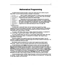
The management-science literature includes several approaches to classifying models. We will begin with a categorization that identifies broad types of models according to the degree of realism that they achieve in representing a given problem. The model categories can be illustrated as shown in Fig. 1.1. Operational Exercise

The first model type is an operational exercise. This modeling approach operates directly with the real environment in which the decision under study is going to take place. The modeling effort merely involves designing a set of experiments to be conducted in that environment, and measuring and interpreting the results of those experiments. Suppose, for instance, that we would like to determine what mix of several crude oils should be blended in a given oil refinery to satisfy, in the most effective way, the market requirements for final products to be delivered from that refinery. If we were to conduct an operational exercise to support that decision, we would try different quantities of several combinations of crude oil types directly in the actual

1.2

Model Classification

3

refinery process, and observe the resulting revenues and costs associated with each alternative mix. After performing quite a few trials, we would begin to develop an understanding of the relationship between the

Fig. 1.1 Types of model representation.

crude oil input and the net revenue obtained from the refinery process, which would guide us in identifying an appropriate mix. In order for this approach to operate successfully, it is mandatory to design experiments to be conducted carefully, to evaluate the experimental results in light of errors that can be introduced by measurement inaccuracies, and to draw inferences about the decisions reached, based upon the limited number of observations performed. Many statistical and optimization methods can be used to accomplish these tasks properly. The essence of the operational exercise is an inductive learning process, characteristic of empirical research in the natural sciences, in which generalizations are drawn from particular observations of a given phenomenon. Operational exercises contain the highest degree of realism of any form of modeling approach, since hardly any external abstractions or oversimplifications are introduced other than those connected with the interpretation of the observed results and the generalizations to be drawn from them. However, the method is exceedingly, usually prohibitively, expensive to implement. Moreover, in most cases it is impossible to exhaustively analyze the alternatives available to the decision-maker. This can lead to severe suboptimization in the final conclusions. For these reasons, operational exercises seldom are used as a pure form of modeling practice. It is important to recognize, however, that direct observation of the actual environment underlies most model conceptualizations and also constitutes one of the most important sources of data. Consequently, even though they may not be used exclusively, operational exercises produce significant contributions to the improvement of managerial decision-making. Gaming

The second type of model in this classification is gaming. In this case, a model is constructed that is an abstract and simplified representation of the real environment. This model provides a responsive mechanism to evaluate the effectiveness of proposed alternatives, which the decision-maker must supply in an organized and sequential fashion. The model is simply a device that allows the decision-maker to test the performance of the various alternatives that seem worthwhile to pursue. In addition, in a gaming situation, all the human interactions that affect the decision environment are allowed to participate actively by providing the inputs they usually are responsible for in the actual realization of their activities. If a gaming approach is used in our previous example, the refinery process would be represented by a computer or mathematical model, which could assume any kind of structure. The model should reflect, with an acceptable degree of accuracy, the relationships between the inputs and outputs of the refinery process. Subsequently, all the personnel who participate in structuring the decision process in the management of the refinery would be allowed to interact with the model. The production manager would establish production plans, the marketing manager would secure contracts and develop marketing

4


1.2

strategies, the purchasing manager would identify prices and sources of crude oil and develop acquisition programs, and so forth. As before, several combinations of quantities and types of crude oil would be tried, and the resulting revenues and cost figures derived from the model would be obtained, to guide us in formulating an optimal policy. Certainly, we have lost some degree of realism in our modeling approach with respect to the operational exercise, since we are operating with an abstract environment, but we have retained some of the human interactions of the real process. However, the cost of processing each alternative has been reduced, and the speed of measuring the performance of each alternative has been increased. Gaming is used mostly as a learning device for developing some appreciation for those complexities inherent in a decision-making process. Several management games have been designed to illustrate how marketing, production, and financial decisions interact in a competitive economy. Simulation

Simulation models are similar to gaming models except that all human decision-makers are removed from the modeling process. The model provides the means to evaluate the performance of a number of alternatives, supplied externally to the model by the decision-maker, without allowing for human interactions at intermediate stages of the model computation. Like operational exercises and gaming, simulation models neither generate alternatives nor produce an optimum answer to the decision under study. These types of models are inductive and empirical in nature; they are useful only to assess the performance of alternatives identified previously by the decision-maker. If we were to conduct a simulation model in our refinery example, we would program in advance a large number of combinations of quantities and types of crude oil to be used, and we would obtain the net revenues associated with each alternative without any external inputs of the decision-makers. Once the model results were produced, new runs could be conducted until we felt that we had reached a proper understanding of the problem on hand. Many simulation models take the form of computer programs, where logical arithmetic operations are performed in a prearranged sequence. It is not necessary, therefore, to define the problem exclusively in analytic terms. This provides an added flexibility in model formulation and permits a high degree of realism to be achieved, which is particularly useful when uncertainties are an important aspect of the decision. Analytical Model

Finally, the fourth model category proposed in this framework is the analytical model. In this type of model, the problem is represented completely in mathematical terms, normally by means of a criterion or objective, which we seek to maximize or minimize, subject to a set of mathematical constraints that portray the conditions under which the decisions have to be made. The model computes an optimal solution, that is, one that satisfies all the constraints and gives the best possible value of the objective function. In the refinery example, the use of an analytical model implies setting up as an objective the maximization of the net revenues obtained from the refinery operation as a function of the types and quantities of the crude oil used. In addition, the technology of the refinery process, the final product requirements, and the crude oil availabilities must be represented in mathematical terms to define the constraints of our problem. The solution to the model will be the exact amount of each available crude-oil type to be processed that will maximize the net revenues within the proposed constraint set. Linear programming has been, in the last two decades, the indisputable analytical model to use for this kind of problem. Analytical models are normally the least expensive and easiest models to develop. However, they introduce the highest degree of simplification in the model representation. As a rule of thumb, it is better to be as much to the right as possible in the model spectrum (no political implication intended!), provided that the resulting degree of realism is appropriate to characterize the decision under study. Most of the work undertaken by management scientists has been oriented toward the development and implementation of analytical models. As a result of this effort, many different techniques and methodologies have been proposed to address specific kinds of problems. Table 1.1 presents a classification of the most important types of analytical and simulation models that have been developed.

1.3

Formulation of Some Examples

5

Table 1.1 Classification of Analytical and Simulation Models Strategy evaluation

Strategy generation

Certainty

Deterministic simulation Econometric models Systems of simultaneous equations Input-output models

Linear programming Network models Integer and mixed-integer programming Nonlinear programming Control theory

Uncertainty

Monte Carlo simulation Econometric models Stochastic processes Queueing theory Reliability theory

Decision theory Dynamic programming Inventory theory Stochastic programming Stochastic control theory

Statistics and subjective assessment are used in all models to determine values for parameters of the models and limits on the alternatives.

The classification presented in Table 1.1 is not rigid, since strategy evaluation models are used for improving decisions by trying different alternatives until one is determined that appears ‘‘best.’’ The important distinction of the proposed classification is that, for strategy evaluation models, the user must first choose and construct the alternative and then evaluate it with the aid of the model. For strategy generation models, the alternative is not completely determined by the user; rather, the class of alternatives is determined by establishing constraints on the decisions, and then an algorithmic procedure is used to automatically generate the ‘‘best’’ alternative within that class. The horizontal classification should be clear, and is introduced because the inclusion of uncertainty (or not) generally makes a substantial difference in the type and complexity of the techniques that are employed. Problems involving uncertainty are inherently more difficult to formulate well and to solve efficiently. This book is devoted to mathematical programming—a part of management science that has a common base of theory and a large range of applications. Generally, mathematical programming includes all of the topics under the heading of strategy generation except for decision theory and control theory. These two topics are entire disciplines in themselves, depending essentially on different underlying theories and techniques. Recently, though, the similarities between mathematical programming and control theory are becoming better understood, and these disciplines are beginning to merge. In mathematical programming, the main body of material that has been developed, and more especially applied, is under the assumption of certainty. Therefore, we concentrate the bulk of our presentation on the topics in the upper righthand corner of Table 1.1. The critical emphasis in the book is on developing those principles and techniques that lead to good formulations of actual decision problems and solution procedures that are efficient for solving these formulations. 1.3

FORMULATION OF SOME EXAMPLES

In order to provide a preliminary understanding of the types of problems to which mathematical programming can be applied, and to illustrate the kind of rationale that should be used in formulating linear-programming problems, we will present in this section three highly simplified examples and their corresponding linearprogramming formulations. Charging a Blast Furnace∗ An iron foundry has a firm order to produce 1000 pounds of castings containing at least 0.45 percent manganese and between 3.25 percent and 5.50 percent silicon. As these particular castings are a special order, there are no suitable castings on hand. The castings sell for $0.45 per pound. The foundry has three types of pig iron available in essentially unlimited amounts, with the following properties: ∗

Excel spreadsheet available at http://web.mit.edu/15.053/www/Sect1.3_Blast_Furnace.xls

6


1.3

Type of pig iron

Silicon Manganese

A

B

4 % 0.45%

1 % 0.5%

C 0.6% 0.4%

Further, the production process is such that pure manganese can also be added directly to the melt. The costs of the various possible inputs are: Pig A Pig B Pig C Manganese

$21/thousand pounds $25/thousand pounds $15/thousand pounds $ 8/pound.

It costs 0.5 cents to melt down a pound of pig iron. Out of what inputs should the foundry produce the castings in order to maximize profits? The first step in formulating a linear program is to define the decision variables of the problem. These are the elements under the control of the decision-maker, and their values determine the solution of the model. In the present example, these variables are simple to identify, and correspond to the number of pounds of pig A, pig B, pig C, and pure manganeseto be used in the production of castings. Specifically, let us denote the decision variables as follows: x1 = Thousands of pounds of pig iron A, x2 = Thousands of pounds of pig iron B, x3 = Thousands of pounds of pig iron C, x4 = Pounds of pure manganese. The next step to be carried out in the formulation of the problem is to determine the criterion the decisionmaker will use to evaluate alternative solutions to the problem. In mathematical-programming terminology, this is known as the objective function. In our case, we want to maximize the total profit resulting from the production of 1000 pounds of castings. Since we are producing exactly 1000 pounds of castings, the total income will be the selling price per pound times 1000 pounds. That is: Total income = 0.45 × 1000 = 450. To determine the total cost incurred in the production of the alloy, we should add the melting cost of $0.005/pound to the corresponding cost of each type of pig iron used. Thus, the relevant unit cost of the pig iron, in dollars per thousand pounds, is: Pig iron A Pig iron B Pig iron C

21 + 5 = 26, 25 + 5 = 30, 15 + 5 = 20.

Therefore, the total cost becomes: Total cost = 26x1 + 30x2 + 20x3 + 8x4 ,

(1)

and the total profit we want to maximize is determined by the expression: Total profit = Total income − Total cost. Thus, Total profit = 450 − 26x1 − 30x2 − 20x3 − 8x4 .

(2)

1.3


7

It is worthwhile noticing in this example that, since the amount of castings to be produced was fixed in advance, equal to 1000 pounds, the maximization of the total profit, given by Eq. (2), becomes completely equivalent to the minimization of the total cost, given by Eq. (1). We should now define the constraints of the problem, which are the restrictions imposed upon the values of the decision variables by the characteristics of the problem under study. First, since the producer does not want to keep any supply of the castings on hand, we should make the total amount to be produced exactly equal to 1000 pounds; that is, 1000x1 + 1000x2 + 1000x3 + x4 = 1000.

(3)

Next, the castings should contain at least 0.45 percent manganese, or 4.5 pounds in the 1000 pounds of castings to be produced. This restriction can be expressed as follows: 4.5x1 + 5.0x2 + 4.0x3 + x4 ≥ 4.5.

(4)

The term 4.5x1 is the pounds of manganese contributed by pig iron A since each 1000 pounds of this pig iron contains 4.5 pounds of manganese. The x2 , x3 , and x4 terms account for the manganese contributed by pig iron B, by pig iron C, and by the addition of pure manganese. Similarly, the restriction regarding the silicon content can be represented by the following inequalities: 40x1 + 10x2 + 6x3 ≥ 32.5, 40x1 + 10x2 + 6x3 ≤ 55.0.

(5) (6)

Constraint (5) establishes that the minimum silicon content in the castings is 3.25 percent, while constraint (6) indicates that the maximum silicon allowed is 5.5 percent. Finally, we have the obvious nonnegativity constraints: x1 ≥ 0,

x2 ≥ 0,

x3 ≥ 0,

x4 ≥ 0.

If we choose to minimize the total cost given by Eq. (1), the resulting linear programming problem can be expressed as follows: Minimize z =

26x1 +

30x2 +

20x3 +

8x4 ,

subject to: 1000x1 4.5x1 40x1 40x1

+ 1000x2 + 1000x3 + + 5.0x2 + 4.0x3 + + 10x2 + 6x3 + 10x2 + 6x3

x1 ≥ 0,

x2 ≥ 0,

x3 ≥ 0,

x4 = 1000, x4 ≥ 4.5, ≥ 32.5, ≤ 55.0, x4 ≥ 0.

Often, this algebraic formulation is represented in tableau form as follows:

Total lbs. Manganese Silicon lower Silicon upper Objective (Optimal solution)

Decision variables x1 x2 x3 x4 1000 1000 1000 1 4.5 5 4 1 40 10 6 0 40 10 6 0 26 30 20 8 0.779 0 0.220 0.111

Relation = ≥ ≥ ≤ =

Requirements 1000 4.5 32.5 55.0 z (min) 25.54

The bottom line of the tableau specifies the optimal solution to this problem. The solution includes the values of the decision variables as well as the minimum cost attained, $25.54 per thousand pounds; this solution was generated using a commercially available linear-programming computer system. The underlying solution procedure, known as the simplex method, will be explained in Chapter 2.

8


1.3

Fig. 1.2 Optimal cost of castings as a function of the cost of pure manganese.

It might be interesting to see how the solution and the optimal value of the objective function is affected by changes in the cost of manganese. In Fig. 1.2 we give the optimal value of the objective function as this cost is varied. Note that if the cost of manganese rises above $9.86/lb., then no pure manganese is used. In the range from $0.019/lb. to $9.86 lb., the values of the decision variables remain unchanged. When manganese becomes extremely inexpensive, less than $0.019/lb., a great deal of manganese is used, in conjuction with only one type of pig iron. Similar analyses can be performed to investigate the behavior of the solution as other parameters of the problem (for example, minimum allowed silicon content) are varied. These results, known as parametric analysis, are reported routinely by commercial linear-programming computer systems. In Chapter 3 we will show how to conduct such analyses in a comprehensive way. Portfolio Selection∗ A portfolio manager in charge of a bank portfolio has $10 million to invest. The securities available for purchase, as well as their respective quality ratings, maturities, and yields, are shown in Table 1.2. Table 1.2 Bond name

Bond type

A B C D E

Municipal Agency Government Government Municipal

Quality scales Moody’s Aa Aa Aaa Aaa Ba

Bank’s 2 2 1 1 5

Years to maturity 9 15 4 3 2

Yield to maturity 4.3% 5.4 5.0 4.4 4.5

After-tax yield 4.3% 2.7 2.5 2.2 4.5

The bank places the following policy limitations on the portfolio manager’s actions: 1. Government and agency bonds must total at least $4 million. 2. The average quality of the portfolio cannot exceed 1.4 on the bank’s quality scale. (Note that a low number on this scale means a high-quality bond.) 3. The average years to maturity of the portfolio must not exceed 5 years. Assuming that the objective of the portfolio manager is to maximize after-tax earnings and that the tax rate is 50 percent, what bonds should he purchase? If it became possible to borrow up to $1 million at 5.5 percent ∗ Excel spreadsheet available at http://web.mit.edu/15.053/www/Sect1.3_Portfolio_Selection.xls

1.3


9

before taxes, how should his selection be changed? Leaving the question of borrowed funds aside for the moment, the decision variables for this problem are simply the dollar amount of each security to be purchased: xA xB xC xD xE

= Amount to be invested in bond A; in millions of dollars. = Amount to be invested in bond B; in millions of dollars. = Amount to be invested in bond C; in millions of dollars. = Amount to be invested in bond D; in millions of dollars. = Amount to be invested in bond E; in millions of dollars.

We must now determine the form of the objective function. Assuming that all securities are purchased at par (face value) and held to maturity and that the income on municipal bonds is tax-exempt, the after-tax earnings are given by: z = 0.043xA + 0.027xB + 0.025xC + 0.022xD + 0.045xE . Now let us consider each of the restrictions of the problem. The portfolio manager has only a total of ten million dollars to invest, and therefore: xA + xB + xC + xD + xE ≤ 10. Further, of this amount at least $4 million must be invested in government and agency bonds. Hence, xB + xC + xD ≥ 4. The average quality of the portfolio, which is given by the ratio of the total quality to the total value of the portfolio, must not exceed 1.4: 2xA + 2xB + xC + xD + 5xE ≤ 1.4. xA + xB + xC + xD + xE Note that the inequality is less-than-or-equal-to, since a low number on the bank’s quality scale means a high-quality bond. By clearing the denominator and re-arranging terms, we find that this inequality is clearly equivalent to the linear constraint: 0.6xA + 0.6xB − 0.4xC − 0.4xD + 3.6xE ≤ 0. The constraint on the average maturity of the portfolio is a similar ratio. The average maturity must not exceed five years: 9xA + 15xB + 4xC + 3xD + 2xE ≤ 5, xA + xB + xC + xD + xE which is equivalent to the linear constraint: 4xA + 10xB − xC − 2xD − 3xE ≤ 0. Note that the two ratio constraints are, in fact, nonlinear constraints, which would require sophisticated computational procedures if included in this form. However, simply multiplying both sides of each ratio constraint by its denominator (which must be nonnegative since it is the sum of nonnegative variables) transforms this nonlinear constraint into a simple linear constraint. We can summarize our formulation in tableau form, as follows: xA xB Cash 1 1 Governments 1 Quality 0.6 0.6 Maturity 4 10 Objective 0.043 0.027 (Optimal solution) 3.36 0

xC 1 1 −0.4 −1 0.025 0

xD 1 1 −0.4 −2 0.022 6.48

xE 1

Relation Limits ≤ 10 ≥ 4 3.6 ≤ 0 −3 ≤ 0 0.045 = z (max) 0.16 0.294

10


1.3

The values of the decision variables and the optimal value of the objective function are again given in the last row of the tableau. Now consider the additional possibility of being able to borrow up to $1 million at 5.5 percent before taxes. Essentially, we can increase our cash supply above ten million by borrowing at an after-tax rate of 2.75 percent. We can define a new decision variable as follows: y = amount borrowed in millions of dollars. There is an upper bound on the amount of funds that can be borrowed, and hence y ≤ 1. The cash constraint is then modified to reflect that the total amount purchased must be less than or equal to the cash that can be made available including borrowing: xA + xB + xC + xD + xE ≤ 10 + y. Now, since the borrowed money costs 2.75 percent after taxes, the new after-tax earnings are: z = 0.043xA + 0.027xB + 0.025xC + 0.022xD + 0.045xE − 0.0275y. We summarize the formulation when borrowing is allowed and give the solution in tableau form as follows: Cash Borrowing Governments Quality Maturity Objective (Optimal solution)

xA 1

xB 1

xC 1

xD 1

xE 1

0.6 4 0.043 3.70

1 0.6 10 0.027 0

1 −0.4 −1 0.025 0

1 −0.4 −2 0.022 7.13

3.6 −3 0.045 0.18

y −1 1

−0.0275 1

Relation ≤ ≤ ≥ ≤ ≤ =

Limits 10 1 4 0 0 z (max) 0.296

Production and Assembly A division of a plastics company manufactures three basic products: sporks, packets, and school packs. A spork is a plastic utensil which purports to be a combination spoon, fork, and knife. The packets consist of a spork, a napkin, and a straw wrapped in cellophane. The school packs are boxes of 100 packets with an additional 10 loose sporks included. Production of 1000 sporks requires 0.8 standard hours of molding machine capacity, 0.2 standard hours of supervisory time, and $2.50 in direct costs. Production of 1000 packets, including 1 spork, 1 napkin, and 1 straw, requires 1.5 standard hours of the packaging-area capacity, 0.5 standard hours of supervisory time, and $4.00 in direct costs. There is an unlimited supply of napkins and straws. Production of 1000 school packs requires 2.5 standard hours of packaging-area capacity, 0.5 standard hours of supervisory time, 10 sporks, 100 packets, and $8.00 in direct costs. Any of the three products may be sold in unlimited quantities at prices of $5.00, $15.00, and $300.00 per thousand, respectively. If there are 200 hours of production time in the coming month, what products, and how much of each, should be manufactured to yield the most profit? The first decision one has to make in formulating a linear programming model is the selection of the proper variables to represent the problem under consideration. In this example there are at least two different sets of variables that can be chosen as decision variables. Let us represent them by x’s and y’s and define them as follows: x1 = Total number of sporks produced in thousands, x2 = Total number of packets produced in thousands, x3 = Total number of school packs produced in thousands,

1.3


11

and y1 = Total number of sporks sold as sporks in thousands, y2 = Total number of packets sold as packets in thousands, y3 = Total number of school packs sold as school packs in thousands. We can determine the relationship between these two groups of variables. Since each packet needs one spork, and each school pack needs ten sporks, the total number of sporks sold as sporks is given by: y1 = x1 − x2 − 10x3 .

(7)

Similarly, for the total number of packets sold as packets we have: y2 = x2 − 100x3 .

(8)

Finally, since all the school packs are sold as such, we have: y3 = x3 .

(9)

From Eqs. (7), (8), and (9) it is easy to express the x’s in terms of the y’s, obtaining: x1 = y1 + y2 + 110y3 , x2 = y2 + 100y3 , x3 = y3 .

(10) (11) (12)

As a matter of exercise, let us formulate the linear program corresponding to the present example in two forms: first, using the x’s as decision variables, and second, using the y’s as decision variables. The objective function is easily determined in terms of both y- and x-variables by using the information provided in the statement of the problem with respect to the selling prices and the direct costs of each of the units produced. The total profit is given by: Total profit = 5y1 + 15y2 + 300y3 − 2.5x1 − 4x2 − 8x3 .

(13)

Equations (7), (8), and (9) allow us to express this total profit in terms of the x-variables alone. After performing the transformation, we get: Total profit = 2.5x1 + 6x2 − 1258x3 .

(14)

Now we have to set up the restrictions imposed by the maximum availability of 200 hours of production time. Since the sporks are the only items requiring time in the injection-molding area, and they consume 0.8 standard hours of production per 1000 sporks, we have: 0.8x1 ≤ 200.

(15)

1.5x2 + 2.5x3 ≤ 200,

(16)

0.2x1 + 0.5x2 + 0.5x3 ≤ 200.

(17)

For packaging-area capacity we have: while supervisory time requires that

In addition to these constraints, we have to make sure that the number of sporks, packets, and school packs sold as such (i.e., the y-variables) are nonnegative. Therefore, we have to add the following constraints: x1 − x2 − 10x3 ≥ 0, x2 − 100x3 ≥ 0, x3 ≥ 0.

(18) (19) (20)

12


1.4

Finally, we have the trivial nonnegativity conditions x1 ≥ 0,

x2 ≥ 0,

x3 ≥ 0.

(21)

Note that, besides the nonnegativity of all the variables, which is a condition always implicit in the methods of solution in linear programming, this form of stating the problem has generated six constraints, (15) to (20). If we expressed the problem in terms of the y-variables, however, conditions (18) to (20) correspond merely to the nonnegativity of the y-variables, and these constraints are automatically guaranteed because the y’s are nonnegative and the x’s expressed by (10), (11), and (12), in terms of the y’s, are the sum of nonnegative variables, and therefore the x’s are always nonnegative. By performing the proper changes of variables, it is easy to see that the linear-programming formulation in terms of the y-variables is given in tableau form as follows: Molding Packaging Supervisory Objective (Optimal solution)

y1 0.8 0.2 2.5 116.7

y2 0.8 1.5 0.7 8.5 133.3

y3 88 152.5 72.5 −383 0

Relation ≤ ≤ ≤ =

Limits 200 200 200 z (max) 1425

Since the computation time required to solve a linear programming problem increases roughly with the cube of the number of rows of the problem, in this example the y’s constitute better decision variables than the x’s. The values of the x’s are easily determined from Eqs. (10), (11), and (12). 1.4

A GEOMETRICAL PREVIEW

Although in this introductory chapter we are not going to discuss the details of computational procedures for solving mathematical programming problems, we can gain some useful insight into the characteristics of the procedures by looking at the geometry of a few simple examples. Since we want to be able to draw simple graphs depicting various possible situations, the problem initially considered has only two decision variables. The Problem∗ Suppose that a custom molder has one injection-molding machine and two different dies to fit the machine. Due to differences in number of cavities and cycle times, with the first die he can produce 100 cases of six-ounce juice glasses in six hours, while with the second die he can produce 100 cases of ten-ounce fancy cocktail glasses in five hours. He prefers to operate only on a schedule of 60 hours of production per week. He stores the week’s production in his own stockroom where he has an effective capacity of 15,000 cubic feet. A case of six-ounce juice glasses requires 10 cubic feet of storage space, while a case of ten-ounce cocktail glasses requires 20 cubic feet due to special packaging. The contribution of the six-ounce juice glasses is $5.00 per case; however, the only customer available will not accept more than 800 cases per week. The contribution of the ten-ounce cocktail glasses is $4.50 per case and there is no limit on the amount that can be sold. How many cases of each type of glass should be produced each week in order to maximize the total contribution? Formulation of the Problem

We first define the decision variables and the units in which they are measured. For this problem we are interested in knowing the optimal number of cases of each type of glass to produce per week. Let x1 = Number of cases of six-ounce juice glasses produced per week (in hundreds of cases per week), and x2 = Number of cases of ten-ounce cocktail glasses produced per week (in hundreds of cases per week). ∗

Excel spreadsheet available at http://web.mit.edu/15.053/www/Sect1.4_Glass_Problem.xls

1.4

A Geometrical Preview

13

The objective function is easy to establish since we merely want to maximize the contribution to overhead, which is given by: Contribution = 500x1 + 450x2 , since the decision variables are measured in hundreds of cases per week. We can write the constraints in a straightforward manner. Because the custom molder is limited to 60 hours per week, and production of six-ounce juice glasses requires 6 hours per hundred cases while production of ten-ounce cocktail glasses requires 5 hours per hundred cases, the constraint imposed on production capacity in units of production hours per week is: 6x1 + 5x2 ≤ 60. Now since the custom molder has only 15,000 cubic feet of effective storage space and a case of six-ounce juice glasses requires 10 cubic feet, while a case of ten-ounce cocktail glasses requires 20 cubic feet, the constraint on storage capacity, in units of hundreds of cubic feet of space per week, is: 10x1 + 20x2 ≤ 150. Finally, the demand is such that no more than 800 cases of six-ounce juice glasses can be sold each week. Hence, x1 ≤ 8. Since the decision variables must be nonnegative, x1 ≥ 0,

x2 ≥ 0,

and we have the following linear program: Maximize z = 500x1 + 450x2 , subject to: 6x1 + 5x2 ≤ 60 10x1 + 20x2 ≤ 150 x1 ≤ 8 x1 ≥ 0,

(production hours) (hundred sq. ft. storage) (sales limit 6 oz. glasses)

x2 ≥ 0.

Graphical Representation of the Decision Space

We now look at the constraints of the above linear-programming problem. All of the values of the decision variables x1 and x2 that simultaneously satisfy these constraints can be represented geometrically by the shaded area given in Fig. 1.3. Note that each line in this figure is represented by a constraint expressed as an equality. The arrows associated with each line show the direction indicated by the inequality sign in each constraint. The set of values of the decision variables x1 and x2 that simultaneously satisfy all the constraints indicated by the shaded area are the feasible production possibilities or feasible solutions to the problem. Any production alternative not within the feasible region must violate at least one of the constraints of the problem. Among these feasible production alternatives, we want to find the values of the decision variables x1 and x2 that maximize the resulting contribution to overhead. Finding an Optimal Solution

To find an optimal solution we first note that any point in the interior of the feasible region cannot be an optimal solution since the contribution can be increased by increasing either x1 or x2 or both. To make this point more clearly, let us rewrite the objective function z = 500x1 + 450x2 ,

14


1.4

Fig. 1.3 Graphical representation of the feasible region.

in terms of x2 as follows: 1 x2 = z− 450

500 x1 . 450

1 If z is held fixed at a given constant value, this expression represents a straight line, where 450 z is the intercept with the x2 axis (i.e., the value of x2 when x1 = 0), and − 500 is the slope (i.e., the change in the 450 value of x2 corresponding to a unit increase in the value of x1 ). Note that the slope of this straight line is constant, independent of the value of z. As the value of z increases, the resulting straight lines move parallel 1 to themselves in a northeasterly direction away from the origin (since the intercept 450 z increases when z 500 increases, and the slope is constant at − 450 ). Figure 1.4 shows some of these parallel lines for specific values of z. At the point labeled P1, the line intercepts the farthest point from the origin within the feasible region, and the contribution z cannot be increased any more. Therefore, point P1 represents the optimalsolution. Since reading the graph may be difficult, we can compute the values of the decision variables by recognizing that point P1 is determined by the intersection of the production-capacity constraint and the storage-capacity constraint. Solving these constraints,

6x1 + 5x2 = 60, 10x1 + 20x2 = 150, yields x1 = 6 73 , x2 = 4 27 ; and substituting these values into the objective function yields z = 5142 67 as the maximum contribution that can be attained. Note that the optimal solution is at a corner point, or vertex, of the feasible region. This turns out to be a general property of linear programming: if a problem has an optimal solution, there is always a vertex that is optimal. The simplex method for finding an optimal solution to a general linear program exploits this property by starting at a vertex and moving from vertex to vertex, improving the value of the objective function with each move. In Fig. 1.4, the values of the decision variables and the associated value of the objective function are given for each vertex of the feasible region. Any procedure that starts at one of the vertices and looks for an improvement among adjacent vertices would also result in the solution labeled P1. An optimal solution of a linear program in its simplest form gives the value of the criterion function, the levels of the decision variables, and the amount of slack or surplus in the constraints. In the custom-molder

1.4


15

Fig. 1.4 Finding the optimal solution.

example, the criterion was maximum contribution, which turned out to be z = $5142 67 ; the levels of the decision variables are x1 = 6 73 hundred cases of six-ounce juice glasses and x2 = 4 27 hundred cases of ten-ounce cocktail glasses. Only the constraint on demand for six-ounce juice glasses has slack in it, since the custom molder could have chosen to make an additional 1 47 hundred cases if he had wanted to decrease the production of ten-ounce cocktail glasses appropriately. Shadow Prices on the Constraints

Solving a linear program usually provides more information about an optimal solution than merely the values of the decision variables. Associated with an optimal solution are shadow prices (also referred to as dual variables, marginal values, or pi values) for the constraints. The shadow price on a particular constraint represents the change in the value of the objective function per unit increase in the righthand-side value of that constraint. For example, suppose that the number of hours of molding-machine capacity was increased from 60 hours to 61 hours. What is the change in the value of the objective function from such an increase? Since the constraints on production capacity and storage capacity remain binding with this increase, we need only solve 6x1 + 5x2 = 61, 10x1 + 20x2 = 150, to find a new optimal solution. The new values of the decision variables are x1 = 6 57 and x2 = 4 17 , and the new value of the objective function is: z = 500x1 + 450x2 = 500 6 57 + 450 4 17 = 5,221 37 . The shadow price associated with the constraint on production capacity then becomes: 5221 37 − 5142 67 = 78 47 . The shadow price associated with production capacity is $78 47 per additional hour of production time. This is important information since it implies that it would be profitable to invest up to $78 47 each week to increase production time by one hour. Note that the units of the shadow price are determined by the ratio of the units of the objective function and the units of the particular constraint under consideration.

16


1.4

Fig. 1.5 Range on the slope of the objective function.

We can perform a similar calculation to find the shadow price 2 67 associated with the storage-capacity constraint, implying that an addition of one hundred cubic feet of storage capacity is worth $2 67 . The shadow price associated with the demand for six-ounce juice glasses clearly must be zero. Since currently we are not producing up to the 800-case limit, increasing this limit will certainly not change our decision and therefore will not be of any value. Finally, we must consider the shadow prices associated with the nonnegativity constraints. These shadow prices often are called the reduced costs and usually are reported separately from the shadow prices on the other constraints; however, they have the identical interpretation. For our problem, increasing either of the nonnegativity constraints separately will not affect the optimal solution, so the values of the shadow prices, or reduced costs, are zero for both nonnegativity constraints. Objective and Righthand-Side Ranges

The data for a linear program may not be known with certainty or may be subject to change. When solving linear programs, then, it is natural to ask about the sensitivity of the optimal solution to variations in the data. For example, over what range can a particular objective-function coefficient vary without changing the optimal solution? It is clear from Fig. 1.5 that some variation of the contribution coefficients is possible without a change in the optimal levels of the decision variables. Throughout our discussion of shadow prices, we assumed that the constraints defining the optimal solution did not change when the values of their righthand sides were varied. Further, when we made changes in the righthand-side values we made them one at a time, leaving the remaining coefficients and values in the problem unchanged. The question naturally arises, over what range can a particular righthand-side value change without changing the shadow prices associated with that constraint? These questions of simple one-at-a-time changes in either the objective-function coefficients or the right-hand-side values are determined easily and therefore usually are reported in any computer solution.

Changes in the Coefficients of the Objective Function

We will consider first the question of making one-at-a-time changes in the coefficients of the objective function. Suppose we consider the contribution per one hundred cases of six-ounce juice glasses, and determine the range for that coefficient such that the optimal solution remains unchanged. From Fig. 1.5, it should be clear that the optimal solution remains unchanged as long as the slope of the objective function lies between the

1.4


17

slope of the constraint on production capacity and the slope of the constraint on storage capacity. We can determine the range on the coefficient of contribution from six-ounce juice glasses, which we denote by c1 , by merely equating the respective slopes. Assuming the remaining coefficients and values in the problem remain unchanged, we must have: Production slope ≤ Objective slope ≤ Storage slope. Since z = c1 x1 + 450x2 can be written as x2 = (z/450) − (c1 /450)x1 , we see, as before, that the objective slope is −(c1 /450). Thus c1 1 6 ≤− − ≤− 5 450 2 or, equivalently, 225 ≤ c1 ≤ 540, where the current values of c1 = 500. Similarly, by holding c1 fixed at 500, we can determine the range of the coefficient of contribution from ten-ounce cocktail glasses, which we denote by c2 : 6 500 1 − ≤− ≤− 5 c2 2 or, equivalently, 416 23 ≤ c2 ≤ 1000, where the current value of c2 = 450. The objective ranges are therefore the range over which a particular objective coefficient can be varied, all other coefficients and values in the problem remaining unchanged, and have the optimal solution (i.e., levels of the decision variables) remain unchanged. From Fig. 1.5 it is clear that the same binding constraints will define the optimal solution. Although the levels of the decision variables remain unchanged, the value of the objective function, and therefore the shadow prices, will change as the objective-function coefficients are varied. It should now be clear that an optimal solution to a linear program is not always unique. If the objective function is parallel to one of the binding constraints, then there is an entire set of optimal solutions. Suppose that the objective function were z = 540x1 + 450x2 . It would be parallel to the line determined by the production-capacity constraint; and all levels of the decision variables lying on the line segment joining the points labeled P1 and P2 in Fig. 1.6 would be optimal solutions.

Changes in the Righthand-Side Values of the Constraints

Now consider the question of making one-at-a-time changes in the righthand-side values of the constraints. Suppose that we want to find the range on the number of hours of production capacity that will leave all of the shadow prices unchanged. The essence of our procedure for computing the shadow prices was to assume that the constraints defining the optimal solution would remain the same even though a righthand-side value was being changed. First, let us consider increasing the number of hours of production capacity. How much can the production capacity be increased and still give us an increase of $78 47 per hour of increase? Looking at Fig. 1.7, we see that we cannot usefully increase production capacity beyond the point where storage capacity and the limit on demand for six-ounce juice glasses become binding. This point is labeled P3 in Fig. 1.7. Any further increase in production hours would be worth zero since they would go unused. We can determine the number of hours of production capacity corresponding to the point labeled P3, since this point

18


1.4

Fig. 1.6 Objective function coincides with a constraint.

Fig. 1.7 Ranges on the righthand-side values.

is characterized by x1 = 8 and x2 = 3 21 . Hence, the upper bound on the range of the righthand-side value for production capacity is 6(8) + 5(3 21 ) = 65 21 hours. Alternatively, let us see how much the capacity can be decreased before the shadow prices change. Again looking at Fig. 1.7, we see that we can decrease production capacity to the point where the constraint on storage capacity and the nonnegativity constraint on ten-ounce cocktail glasses become binding. This point is labeled P4 in Fig. 1.7 and corresponds to only 37 21 hours of production time per week, since x1 = 0 and x2 = 7 21 . Any further decreases in production capacity beyond this point would result in lost contribution of $90 per hour of further reduction. This is true since at this point it is optimal just to produce as many cases of the ten-ounce cocktail glasses as possible while producing no six-ounce juice glasses at all. Each hour of reduced production time now causes a reduction of 15 of one hundred cases of ten-ounce cocktail glasses valued at $450, i.e., 15 (450) = 90. Hence, the range over which the shadow prices remain unchanged is the range over which the optimal solution is defined by the same binding constraints. If we take the righthandside value of production capacity to be b1 , the range on this value, such that the shadow prices will remain

1.4


19

unchanged, is: 37 21 ≤ b1 ≤ 65 21 , where the current value of production capacity b1 = 60 hours. It should be emphasized again that this righthand-side range assumes that all other righthand-side values and all variable coefficients in the problem remain unchanged. In a similar manner we can determine the ranges on the righthand-side values of the remaining constraints: 128 ≤ b2 ≤ 240, 6 37 ≤ b3 . Observe that there is no upper bound on six-ounce juice-glass demand b3 , since this constraint is nonbinding at the current optional solution P1. We have seen that both cost and righthand-side ranges are valid if the coefficient or value is varied by itself, all other variable coefficients and righthand-side values being held constant. The objective ranges are the ranges on the coefficients of the objective function, varied one at a time, such that the levels of the decision variables remain unchanged in the optimal solution. The righthand-side ranges are the ranges on the righthand-side values, varied one at a time, such that the shadow prices associated with the optimal solution remain unchanged. In both instances, the ranges are defined so that the binding constraints at the optimal solution remain unchanged. Computational Considerations

Until now we have described a number of the properties of an optimal solution to a linear program, assuming first that there was such a solution and second that we were able to find it. It could happen that a linear program has no feasible solution. An infeasible linear program might result from a poorly formulated problem, or from a situation where requirements exceed the capacity of the existing available resources. Suppose, for example, that an additional constraint was added to the model imposing a minimum on the number of production hours worked. However, in recording the data, an error was made that resulted in the following constraint being included in the formulation: 6x1 + 5x2 ≥ 80. The graphical representation of this error is given in Fig. 1.8. The shading indicates the direction of the inequalities associated with each constraint. Clearly, there are no points that satisfy all the constraints simultaneously, and the problem is therefore infeasible. Computer routines for solving linear programs must be able to tell the user when a situation of this sort occurs. In general, on large problems it is relatively easy to have infeasibilities in the initial formulation and not know it. Once these infeasibilities are detected, the formulation is corrected. Another type of error that can occur is somewhat less obvious but potentially more costly. Suppose that we consider our original custom-molder problem but that a control message was typed into the computer incorrectly so that we are, in fact, attempting to solve our linear program with ‘‘greater than or equal to’’ constraints instead of ‘‘less than or equal to’’ constraints. We would then have the following linear program: Maximize z = 500x1 + 450x2 , subject to: 6x1 + 5x2 ≥ 60, 10x1 + 20x2 ≥ 150, x1 ≥ 8, x1 ≥ 0, x2 ≥ 0. The graphical representation of this error is given in Fig. 1.9.

20


1.4

Fig. 1.8 An infeasible group of constraints.

Clearly, the maximum of the objective function is now unbounded. That is, we apparently can make our contribution arbitrarily large by increasing either x1 or x2 . Linear-programming solution procedures also detect when this kind of error has been made, and automatically terminate the calculations indicating the direction that produces the unbounded objective value. Integer Solutions

In linear programming, the decision space is continuous, in the sense that fractional answers always are allowed. This is contrasted with discrete or integer programming, where integer values are required for some or all variables. In our custom-molding example, if the customer will accept each product only in even hundred-case lots, in order to ease his reordering situation, and if, further, we choose not to store either product from one week to the next, we must seek an integer solution to our problem. Our initial reaction is to round off our continuous solution, yielding x1 = 6,

x2 = 4,

which in this case is feasible, since we are rounding down. The resulting value of contribution is z = $4800. Is this the optimal integer solution? We clearly could increase the total contribution if we could round either x1 or x2 up instead of down. However, neither the point x1 = 7, x2 = 4, nor the point x1 = 6, x2 = 5 is within the feasible region. Another alternative would be to start with our trial solution x1 = 6, x2 = 4, and examine ‘‘nearby’’ solutions such as x1 = 5, x2 = 5, which turns out to be feasible and which has a contribution of z = $4750, not as high as our trial solution. Another ‘‘nearby’’ solution is x1 = 7, x2 = 3, which is also feasible and has a contribution z = $4850. Since this integer solution has a higher contribution than any previous integer solution, we can use it as our new trial solution. It turns out that the optimal integer solution for our problem is: x1 = 8, x2 = 2, with a contribution of z = $4900. It is interesting to note that this solution is not particularly ‘‘nearby’’ the optimal continuous solution x1 = 6 73 , x2 = 4 27 .

1.4


21

Fig. 1.9 An unbounded solution.

Basically, the integer-programming problem is inherently difficult to solve and falls in the domain of combinatorial analysis rather than simple linear programming. Special algorithms have been developed to find optimal integer solutions; however, the size of problem that can be solved successfully by these algorithms is an order of magnitude smaller than the size of linear programs that can easily be solved. Whenever it is possible to avoid integer variables, it is usually a good idea to do so. Often what at first glance seem to be integer variables can be interpreted as production or operating rates, and then the integer difficulty disappears. In our example, if it is not necessary to ship in even hundred-case lots, or if the odd lots are shipped the following week, then it still is possible to produce at rates x1 = 6 73 and x2 = 4 27 hundred cases per week. Finally, in any problem where the numbers involved are large, rounding to a feasible integer solution usually results in a good approximation. Nonlinear Functions

In linear programming the variables are continuous and the functions involved are linear. Let us now consider the decision problem of the custom molder in a slightly altered form. Suppose that the interpretation of production in terms of rates is acceptable, so that we need not find an integer solution; however, we now have a nonlinear objective function. We assume that the injection-molding machine is fairly old and that operating near capacity results in a reduction in contribution per unit for each additional unit produced, due to higher maintenance costs and downtime. Assume that the reduction is $0.05 per case of six-ounce juice glasses and $0.04 per case of ten-ounce cocktail glasses. In fact, let us assume that we have fit the following functions to per-unit contribution for each type of glass: z 1 (x1 ) = 60 − 5x1 z 2 (x2 ) = 80 − 4x2

for six-ounce juice glasses, for ten-ounce cocktail glasses.

The resulting total contribution is then given by: (60 − 5x1 )x1 + (80 − 4x2 )x2 . Hence, we have the following nonlinear programming problem to solve: Maximize z = 60x1 −

5x12 + 80x2 − 4x22 ,

22


subject to:

1.5

6x1 + 5x2 ≤ 60, 10x1 + 20x2 ≤ 150, x1 ≤ 8, x1 ≥ 0,

x2 ≥ 0.

This situation is depicted in Fig. 1.10. The curved lines represent lines of constant contribution. Note that the optimal solution is no longer at a corner point of the feasible region. This property alone makes finding an optimal solution much more difficult than in linear programming. In this situation, we cannot merely move from vertex to vertex, looking for an improvement at each iteration. However, this particular problem has the property that, if you have a trial solution and cannot find an improving direction to move in, then the trial solution is an optimal solution. It is this property that is generally exploited in computational procedures for nonlinear programs.

Fig. 1.10 The nonlinear program. 1.5

A CLASSIFICATION OF MATHEMATICAL PROGRAMMING MODELS

We are now in a position to provide a general statement of the mathematical programming problem and formally summarize definitions and notation introduced previously. Let us begin by giving a formal representation of the general linear programming model. In mathematical terms, the linear programming model can be expressed as the maximization (or minimization) of an objective (or criterion) function, subject to a given set of linear constraints. Specifically, the linear programming problem can be described as finding the values of n decision variables, x1 , x2 , . . . , xn , such that they maximize the objective function z where z = c1 x 1 + c2 x 2 + · · · + cn x n , subject to the following constraints: a11 x1 + a12 x2 + · · · + a1n xn ≤ b1 , a21 x1 + a22 x2 + · · · + a2n xn ≤ b2 , .. .. . . am1 x1 + am2 x2 + · · · + amn xn ≤ bm , and, usually, x1 ≥ 0, x2 ≥ 0, ..., xn ≥ 0,

(22)

(23)

(24)

1.5

A Classification of Mathematical Programming Models

23

where c j , ai j , and bi are given constants. It is easy to provide an immediate interpretation to the general linear-programming problem just stated in terms of a production problem. For instance, we could assume that, in a given production facility, there are n possible products we may manufacture; for each of these we want to determine the level of production which we shall designate by x1 , x2 , . . . , xn . In addition, these products compete for m limited resources, which could be manpower availability, machine capacities, product demand, working capital, and so forth, and are designated by b1 , b2 , . . . , bm . Let ai j be the amount of resource i required by product j and let c j be the unit profit of product j. Then the linear-programming model seeks to determine the production quantity of each product in such a way as to maximize the total resulting profit z (Eq. 22), given that the available resources should not be exceeded (constraints 23), and that we can produce only positive or zero amounts of each product (constraints 24). Linear programming is not restricted to the structure of the problem presented above. First, it is perfectly possible to minimize, rather than maximize, the objective function. In addition, ‘‘greater than or equal to’’ or ‘‘equal to’’ constraints can be handled simultaneously with the ‘‘less than or equal to’’ constraints presented in constraints (23). Finally, some of the variables may assume both positive and negative values. There is some technical terminology associated with mathematical programming, informally introduced in the previous section, which we will now define in more precise terms. Values of the decision variables x1 , x2 , . . . , xn that satisfy all the constraints of (23) and (24) simultaneously are said to form a feasible solution to the linear programming problem. The set of all values of the decision variables characterized by constraints (23) and (24) form the feasible region of the problem under consideration. A feasible solution that in addition optimizes the objective function (22) is called an optimal feasible solution. As we have seen in the geometric representation of the problem, solving a linear program can result in three possible situations. i) The linear program could be infeasible, meaning that there are no values of the decision variables x1 , x2 , . . . , xn that simultaneously satisfy all the constraints of (23) and (24). ii) It could have an unbounded solution, meaning that, if we are maximizing, the value of the objective function can be increased indefinitely without violating any of the constraints. (If we are minimizing, the value of the objective function may be decreased indefinitely.) iii) In most cases, it will have at least one finite optimal solution and often it will have multiple optimal solutions. The simplex method for solving linear programs, which will be discussed in Chapter 2, provides an efficient procedure for constructing an optimal solution, if one exists, or for determining whether the problem is infeasible or unbounded. Note that, in the linear programming formulation, the decision variables are allowed to take any continuous value. For instance, values such that x1 = 1.5, x2 = 2.33, are perfectly acceptable as long as they satisfy constraints (23) and (24). An important extension of this linear programming model is to require that all or some of the decision variables be restricted to be integers. Another fundamental extension of the above model is to allow the objective function, or the constraints, or both, to be nonlinear functions. The general nonlinear programming model can be stated as finding the values of the decision variables x1 , x2 , . . . , xn that maximize the objective function z where z = f 0 (x1 , x2 , . . . , xn ),

(25)

f 1 (x1 , x2 , . . . , xn ) ≤ b1 , f 2 (x1 , x2 , . . . , xn ) ≤ b2 , .. . f m (x1 , x2 , . . . , xn ) ≤ bm ,

(26)

subject to the following constraints:

24


and sometimes x1 ≥ 0,

x2 ≥ 0,

...,

xn ≥ 0.

(27)

Often in nonlinear programming the righthand-side values are included in the definition of the function f i (x1 , x2 , . . . , xn ), leaving the righthand side zero. In order to solve a nonlinear programming problem, some assumptions must be made about the shape and behavior of the functions involved. We will leave the specifics of these assumptions until later. Suffice it to say that the nonlinear functions must be rather well-behaved in order to have computationally efficient means of finding a solution. Optimization models can be subject to various classifications depending on the point of view we adopt. According to the number of time periods considered in the model, optimization models can be classified as static (single time period) or multistage (multiple time periods). Even when all relationships are linear, if several time periods are incorporated in the model the resulting linear program could become prohibitively large for solution by standard computational methods. Fortunately, in most of these cases, the problem exhibits some form of special structure that can be adequately exploited by the application of special types of mathematical programming methods. Dynamic programming, which is discussed in Chapter 11, is one approach for solving multistage problems. Further, there is a considerable research effort underway today, in the field of large-scale linear programming, to develop special algorithms to deal with multistage problems. Chapter 12 addresses these issues. Another important way of classifying optimization models refers to the behavior of the parameters of the model. If the parameters are known constants, the optimization model is said to be deterministic. If the parameters are specified as uncertain quantities, whose values are characterized by probability distributions, the optimization model is said to be stochastic. Finally, if some of the parameters are allowed to vary systematically, and the changes in the optimum solution corresponding to changes in those parameters are determined, the optimization model is said to be parametric. In general, stochastic and parametric mathematical programming give rise to much more difficult problems than deterministic mathematical programming. Although important theoretical and practical contributions have been made in the areas of stochastic and parametric programming, there are still no effective general procedures that cope with these problems. Deterministic linear programming, however, can be efficiently applied to very large problems of up to 5000 rows and an almost unlimited number of variables. Moreover, in linear programming, sensitivity analysis and parametric programming can be conducted effectively after obtaining the deterministic optimum solution, as will be seen in Chapter 3. A third way of classifying optimization models deals with the behavior of the variables in the optimal solution. If the variables are allowed to take any value that satisfies the constraints, the optimization model is said to be continuous. If the variables are allowed to take on only discrete values, the optimization model is called integer or discrete. Finally, when there are some integer variables and some continuous variables in the problem, the optimization model is said to be mixed. In general, problems with integer variables are significantly more difficult to solve than those with continuous variables. Network models, which are discussed in Chapter 8, are a class of linear programming models that are an exception to this rule, as their special structure results in integer optimal solutions. Although significant progress has been made in the general area of mixed and integer linear programming, there is still no algorithm that can efficiently solve all general medium-size integer linear programs in a reasonable amount of time though, for special problems, adequate computational techniques have been developed. Chapter 9 comments on the various methods available to solve integer programming problems.

EXERCISES

1. Indicate graphically whether each of the following linear programs has a feasible solution. Graphically determine the optimal solution, if one exists, or show that none exists. a)

Maximize z = x1 + 2x2 ,

Exercises

25

subject to: x1 − 2x2 ≤ 3, x1 + x2 ≤ 3, x1 ≥ 0, b)

x2 ≥ 0.

Minimize z = x1 + x2 , subject to: x1 − x2 ≤ 2, x1 − x2 ≥ −2, x1 ≥ 0,

x2 ≥ 0.

c) Redo (b) with the objective function Maximize z = x1 + x2 . d)

Maximize z = 3x1 + 4x2 , subject to: x1 − 2x2 ≥ 4, x1 + x2 ≤ 3, x1 ≥ 0,

x2 ≥ 0.

2. Consider the following linear program: Maximize z = 2x1 +

x2 ,

subject to: 12x1 + 3x2 ≤ 6, −3x1 + x2 ≤ 7, x2 ≤ 10, x1 ≥ 0,

x2 ≥ 0.

a) Draw a graph of the constraints and shade in the feasible region. Label the vertices of this region with their coordinates. b) Using the graph obtained in (a), find the optimal solution and the maximum value of the objective function. c) What is the slack in each of the constraints? d) Find the shadow prices on each of the constraints. e) Find the ranges associated with the two coefficients of the objective function. f) Find the righthand-side ranges for the three constraints. 3. Consider the bond-portfolio problem formulated in Section 1.3. Reformulate the problem restricting the bonds available only to bonds A and D. Further add a constraint that the holdings of municipal bonds must be less than or equal to $3 million. a) What is the optimal solution? b) What is the shadow price on the municipal limit? c) How much can the municipal limit be relaxed before it becomes a nonbinding constraint? d) Below what interest rate is it favorable to borrow funds to increase the overall size of the portfolio? e) Why is this rate less than the earnings rate on the portfolio as a whole? 4. A liquor company produces and sells two kinds of liquor: blended whiskey and bourbon. The company purchases intermediate products in bulk, purifies them by repeated distillation, mixes them, and bottles the final product under their own brand names. In the past, the firm has always been able to sell all that it produced. The firm has been limited by its machine capacity and available cash. The bourbon requires 3 machine hours per bottle while, due to additional blending requirements, the blended whiskey requires 4 hours of machine time per bottle. There are 20,000 machine hours available in the current production period. The direct operating costs, which are principally for labor and materials, are $3.00 per bottle of bourbon and $2.00 per bottle of blended whiskey.

26


The working capital available to finance labor and material is $4000; however, 45% of the bourbon sales revenues and 30% of the blended-whiskey sales revenues from production in the current period will be collected during the current period and be available to finance operations. The selling price to the distributor is $6 per bottle of bourbon and $5.40 per bottle of blended whiskey. a) Formulate a linear program that maximizes contribution subject to limitations on machine capacity and working capital. b) What is the optimal production mix to schedule? c) Can the selling prices change without changing the optimal production mix? d) Suppose that the company could spend $400 to repair some machinery and increase its available machine hours by 2000 hours. Should the investment be made? e) What interest rate could the company afford to pay to borrow funds to finance its operations during the current period? 5. The truck-assembly division of a large company produces two different models: the Aztec and the Bronco. Their basic operation consists of separate assembly departments: drive-train, coachwork, Aztec final, and Bronco final. The drive-train assembly capacity is limited to a total of 4000 units per month, of either Aztecs or Broncos, since it takes the same amount of time to assemble each. The coachwork capacity each month is either 3000 Aztecs or 6000 Broncos. The Aztecs, which are vans, take twice as much time for coachwork as the Broncos, which are pickups. The final assembly of each model is done in separate departments because of the parts availability system. The division can do the final assembly of up to 2500 Aztecs and 3000 Broncos each month. The profit per unit on each model is computed by the firm as follows: Aztec Selling Price Material cost Labor cost

$2300 400

Gross Margin Selling & Administrative∗ Depreciation† Fixed overhead† Variable overhead

$ 210 60 50 590

Bronco

$4200 2700

$4000 $2000 450

$1500

Profit before taxes

910

2450 $1550

$ 200 180 150 750

$ 590

1280 $ 270

∗ 5% of selling price. † Allocated according to planned production of 1000 Aztecs and 3000 Broncos per monthfor the coming year.

a) Formulate a linear program to aid management in deciding how many trucks of each type to produce per month. b) What is the proper objective function for the division? c) How many Aztecs and Broncos should the division produce each month? 6. Suppose that the division described in Exercise 5 now has the opportunity to increase its drive-train capacity by subcontracting some of this assembly work to a nearby firm. The drive-train assembly department cost breakdown per unit is as follows:

Direct labor Fixed overhead Variable overhead

Aztec

Bronco

$ 80 20 200

$ 60 60 150

$300 $270 The subcontractor will pick up the parts and deliver the assembled drive-trains back to the division. What is the maximum amount that the division would be willing to pay the subcontractor for assembly of each type of drive-train?

Exercises

27

7. Suppose that the division described in Exercises 5 and 6 has decided against subcontracting the assembly of drivetrains but now is considering assembling drive-trains on overtime. If there is a 50% overtime labor premium on each drive-train assembled on overtime and increased fixed overhead of $150,000 per month, should the division go on overtime drive-train production? Formulate a linear program to answer this question, but do not solve explicitly. 8. A manufacturer of wire cloth products can produce four basic product lines: (1) industrial wire cloth; (2) insect screen; (3) roofing mesh; and (4) snow fence. He can sell all that he can produce of each product line for the next year. The production process for each product line is essentially the same. Aluminum wire is purchased in large diameters of approximately 0.375 inches and drawn down to finer diameters of 0.009 to 0.018 inches. Then the fine wire is woven on looms, in much the same manner as textiles. Various types of different wire meshes are produced, depending on product line. For example, industrial wire cloth consists of meshes as fine as 30 wires per inch, while snow fence has approximately 6 wires per inch. The production process is limited by both wire-drawing capacity and weaving capacity, as well as the availability of the basic raw material, large-diameter aluminum wire. For the next planning period, there are 600 hours of wire-drawing machine capacity, 1000 hours of loom capacity, and 15 cwt (hundred weight) of large-diameter aluminum wire. The four product lines require the following inputs to make a thousand square feet of output: Aluminum wire (cwt) Industrial cloth Insect screen Roofing mesh Snow fence

1 3 3 2.5

Wire drawing (100’s of hrs) 1 1 2 1.5

Weaving (100’s of hrs) 2 1 1.5 2

The contributions from industrial cloth, insect screen, roofing mesh, and snow fence are 2.0, 3.0, 4.2, and 4.0, respectively, in 100’s of dollars per thousand square feet. a) Formulate a linear program to maximize the firm’s contribution from the four product lines. b) Since roofing mesh and snow fence are really new product lines, analyze the problem graphically, considering only industrial wire cloth and insect screen. i) What is the optimal solution using only these two product lines? ii) Over what range of contribution of screen cloth will this solution remain optimal? iii) Determine the shadow prices on the resources for this solution. Give an economic interpretation of these shadow prices. iv) Suppose that the manufacturer is considering adding wire-drawing capacity. Over what range of wiredrawing capacity will the shadow price on this constraint remain unchanged? In this range, what happens to the other shadow prices? c) Now, considering the full line of four products, answer the following, making use of the information developed in (b). i) Will it pay to transfer resources into the production of roofing mesh or snow fence? ii) Without performing the calculations, what will be the form of the optimal solution of the full product line? What is the largest number of product lines that will be produced? iii) Suppose that in the future some new product line is developed. Is it possible that one of the product lines not presently included in the optimal solution will then be included? Explain. 9. The Candid Camera Company manufactures three lines of cameras: the Cub, the Quickiematic and the VIP, whose contributions are $3, $9, and $25, respectively. The distribution center requires that at least 250 Cubs, 375 Quickiematics, and 150 VIPs be produced each week. Each camera requires a certain amount of time in order to: (1) manufacture the body parts; (2) assemble the parts (lenses are purchased from outside sources and can be ignored in the production scheduling decision); and (3) inspect, test, and package the final product. The Cub takes 0.1 hours to manufacture, 0.2 hours to assemble, and 0.1 hours to inspect, test, and package. The Quickiematic needs 0.2 hours to manufacture, 0.35 hours to assemble, and 0.2 hours for the final set of operations. The VIP requires 0.7, 0.1, and 0.3 hours, respectively. In addition, there are 250 hours per week of manufacturing time available, 350 hours of assembly, and 150 hours total to inspect, test, and package. Formulate this scheduling problem as a linear program that maximizes contribution.

28


10. A leather-goods factory manufactures five styles of handbags, whose variable contributions are $30, $40, $45, $25, and $60 per dozen, respectively. The products must pass through four work centers and the man-hours available in each are: clicking (700), paring (600), stitching (400), and finishing (900). Hourly requirements for each dozen handbags are: Style 341 262 43 784 5-A

Click

Pare

Stitch

Finish

3 4 2 2 5

8 3 2 1 4

2 1 0 3 4

6 0 2 4 3

To prevent adding to inventory levels already on hand, the production manager, after reviewing the weekly sales forecasts, has specified that no more than 100, 50, 90, 70, and 30 dozen of each style respectively may be produced. Each handbag is made from five materials as specified in the following table: Style

Leather

341 262 43 784 5-A Total available

Fabric

Backing

Lining

Accessories

0 4 5 6 2

1 0 7 4 3

4 7 6 1 3

2 4 2 1 0

3 4 0 2 4

300

400

1000

900

1600

Formulate a linear program for next week’s optimum manufacturing schedule if overall contribution is to be maximized. 11. A corporation that produces gasoline and oil specialty additives purchases three grades of petroleum distillates, A, B, and C. The company then combines the three according to specifications of the maximum or minimum percentages of grades A or C in each blend.

Mixture Deluxe Standard Economy

Max % allowed for Additive A

Min % allowed for Additive C

Selling price $/gallon

60% 15% —

20% 60% 50%

7.9 6.9 5.0

Supplies of the three basic additives and their costs are:

Distillate

Maximum quantity available per day (gals)

Cost $/gallon

A B C

4000 5000 2500

0.60 0.52 0.48

Show how to formulate a linear program to determine the production policy that will maximize profits. 12. Universal Aviation currently is investigating the possibility of branching out from its passenger service into the small-plane air-freight business. With $4,000,000 available to invest in the purchase of new twin-engined cargo aircraft, Universal is considering three types of planes. Aircraft A, costing $80,000, has a ten-ton payload and is expected to cruise at 350 knots, while airplane B can haul 20 tons of goods at an average speed of 300 knots. Aircraft

Exercises

29

B will cost $130,000. The third aircraft is a modified form of B with provisions for a copilot, a 300-knot cruising speed, a reduced capacity of 18 tons, and a cost of $150,000. Plane A requires one pilot and, if flown for three shifts, could average 18 hours a day in the air, as could aircraft B. While transports B and C both require a crew of two, C could average 21 hours of flying per day on a three-shift pilot basis due to superior loading equipment. Universal’s operations department currently estimates that 150 pilot-shifts will be available for each day’s cargo operations. Limitations on maintenance facilities indicate that no more than thirty planes can be purchased. The contributions of planes A, B, and C per ton-mile are, respectively, $1, $8, and $120. 3,500,000 ton-miles of shipping must be completed each day, but deliveries not completed by the in-house fleet can still be sub-contracted to outside air carriers at a contribution of $0.20 per ton mile. What ‘‘mix’’ of aircraft should be purchased if the company desires to maximize its contribution per day? (Note. Consider a knot = 1 mile/hour.) 13. A mobile-home manufacturer in Indiana channels its mobile-home units through distribution centers located in Elkhart, Ind., Albany, N.Y., Camden, N.J., and Petersburg, Va. An examination of their shipping department records indicates that, in the upcoming quarter, the distribution centers will have in inventory 30, 75, 60, and 35 mobile homes, respectively. Quarterly orders submitted by dealerships serviced by the distribution centers require the following numbers of mobile home units for the upcoming quarter: Number of units Dealer A Dealer B Dealer C

25 40 15

Number of units Dealer D Dealer E Dealer F

25 50 45

Transportation costs (in dollars per unit) between each distribution center and the dealerships are as shown in the table below. Dealers Distribution centers Elkhart Albany Camden Petersburg

A 75 90 40 95

B

C

D

E

F

65 30 55 150

175 45 35 100

90 50 80 115

110 105 70 55

150 130 75 55

a) Formulate this problem as a linear-programming problem with the objective of minimizing the transportation costs from the distribution centers to the dealerships. b) Suppose Dealer E had placed an order for 65 units, assuming all other data remain unchanged. How does this affect the problem? (Note that total supply is less than total demand.) 14. A strategic planner for an airline that flies to four different cities from its Boston base owns 10 large jets (B707’s), 15 propeller-driven planes (Electra’s), and two small jets (DC9’s).

Assuming constant flying conditions and passenger usage, the following data is available.

30


B707

Electra

DC9

City

Trip cost*

Trip revenue

A B C D A B C D A B C D

$ 6,000 7,000 8,000 10,000 $ 1,000 2,000 4,000

$ 5,000 7,000 10,000 18,000 $ 3,000 4,000 6,000

$ 2,000 3,500 6,000 10,000

$ 4,000 5,500 8,000 14,000

Average flying time (hours) 1 2 5 10 2 4 8 20 1 2 6 12

* Data is for a round trip. Formulate constraints to take into account the following: i) city D must be served twice daily; cities A, B, and C must be served four times daily; ii) limitation on number of planes available, assuming that each plane can fly at most 18 hours/day. Formulate objective functions for: i) cost minimization; ii) profit maximization; iii) fleet flying-time minimization. Indicate when a continuous linear-programming formulation is acceptable, and when an integer-programming formulation is required. 15. The Temporary Help Company must provide secretaries to its clients over the next year on the following estimated schedule: spring, 6000 secretary-days; summer, 7500 secretary-days; fall, 5500 secretary-days; and winter, 9000 secretary-days. A secretary must be trained for 5 days before becoming eligible for assignment to clients. There are 65 working days in each quarter, and at the beginning of the spring season there are 120 qualified secretaries on the payroll. The secretaries are paid by the company and not the client; they earn a salary of $800 a month. During each quarter, the company loses 15% of its personnel (including secretaries trained in the previous quarter). Formulate the problem as a linear-programming problem. (Hint: Use xt as the number of secretaries hired at the beginning of season t, and St as the total number of secretaries at the beginning of season t.) 16. An imaginary economy has six distinct geographic regions; each has its own specific economic functions, as follows: Region A B C D E F

Function Food producing Manufacturing—Machinery Manufacturing—Machinery and consumer durables Administrative Food-producing Manufacturing—Consumer durables and nondurables

The regions also have the following annual requirements (all quantities measured in tons):

Exercises

Region

Food

Machinery

Consumer durables

Consumer nondurables

A B C D E F

5 15 20 30 10 25

30 100 80 10 60 60

20 40 50 70 30 60

10 30 40 60 20 50

31

Using the national railroad, shipping costs are $1/ton per 100 miles for all hauls over 100 miles. Within 100 miles, all goods are carried by truck at a cost of $1.25/ton per 100 miles ($1/ton minimum charge). The distances (in miles) between regions are as follows:

A B C D E F

A

B

C

D

E

500 200 75 600 300

400 500 125 200

150 350 100

550 400

300

F

Assume producing regions can meet all requirements, but that, due to government regulation, food production in sector A is restricted to half that of sector E. Formulate a linear program that will meet the requirements and minimize the total transportation costs in the economy. 17. The Environmental Protection Agency (EPA) wants to restrict the amount of pollutants added by a company to the river water. The concentrations of phenol and nitrogen in the water are to be restricted to, respectively, P and N lbs. MG (million gallons) on a daily basis. The river has a flow of M MG/day. The company diverts a portion of the river water, adds the pollutants, namely, phenol and nitrogen, to it, and sends the water back to the river. The company has four possible ways to treat the water it uses before returning it to the river. The characteristics of each treatment are given in the following table: (lbs. of pollutant)/MG after treatment Treatment

1

2

3

4

Phenol Nitrogen

P1 N1

P2 N2

P3 N3

P4 N4

Cost/MG

c1

c2

c3

c4

Assume: (i) that the river is initially free of pollutants; (ii) that addition of pollutants does not affect the amount of water flow; and (iii) that the company has to process at least K (MG/day) of river water. a) Set up a linear program to solve for the amount of water to be processed by each treatment, so that total cost of treatment is minimized. b) How does the formulation change if the EPA regulations apply not to total river concentration downstream from the plant, but rather to the concentration of effluent from the plant? 18. Suppose the company of Exercise 17 has three plants, A, B, and C, in a river network as shown below: River water can be clean enough for (1) swimming, or (2) to support bio-life (but not clean enough for swimming). Maximum permissible concentrations of pollutants for both cases are given in the table below.

32


Maximum permissible concentrations (lbs./MG)

Phenol Nitrogen

Swimming

Biological life

PS NS

PB NB

Assume again that each plant has four different alternatives for water treatment, as in the table of Exercise 17, and that A, B, and C must process at least K A , K B , K C MG/day, respectively. It is necessary that water in sections (1) and (3) be clean enough for swimming and that water in section (2) be clean enough to support bio-life. Further, assume: (i) that the river is free of pollutants upstream from plants A and B; and (ii) that adding pollutants does not affect the amount of water flow. a) Formulate a linear program, including plants A, B, and C, that minimizes total treatment costs. b) How would the formulation change if all the plants did not necessarily have the same capabilities and cost structure for each treatment? Indicate modifications only—do not reformulate completely. 19. ‘‘Chemico’’ company produces 3 products from a certain mineral. The production process consists of 2 stages: mining the crude mineral, and processing the mineral to produce 3 different products. The crude mineral can be mined by one of 5 methods. The quality of the mineral depends on the method used and is measured by the percentage of the quantity of the final products that are produced from 1 ton of crude mineral. Furthermore, the distribution of products obtained from 1 ton of crude mineral depends on the mining method used. A limited amount of the crude mineral can be mined by each method. In addition, the capacity of the production process is limited to 850 tons of crude mineral. The following table gives the relevant data. Mining Cost (per ton of No. of hours Mining final products) per 1 ton of Mine Method ($) final products A 1 250 50 2 320 62 3 260 63 B 4 210 55 5 350 60

Quality 65% 80% 76% 76% 78%

Production Production capacity Distribution (tons of Product Product Product crude material) I II III 300 20% 30% 50% 280 25% 35% 40% 400 15% 45% 40% 250 7% 24% 69% 500 35% 40% 25%

Note that the mining costs are per 1 ton of final products, and not per 1 ton of crude mineral. The production capacity of each mining method is in terms of crude material. There are 2 mines: Mine A uses methods 1 and 2, whereas Mine B uses methods 3, 4, and 5. The total number of work hours available in Mines A and B are 13,000 and 15,000, respectively (for the planning period). It is possible to transfer workers from A to B and vice versa, but it costs $2 to transfer 1 work hour, and 10% of the transferred work hours are wasted. The company sells its products in 5 markets. The selling price depends on the market, and in each market the amount that can be sold is limited. The relevant data are given in a second table:

Exercises

Market

Product

Price per 1 ton ($)

Max. amount (tons)

1

I

1550

150

2

I

1600

100

3

II

1400

200

4

III

1000

50

5

III

850

400

33

Management wants to plan the production for the next period such that the profit will be maximized. They want to know how many work hours to assign to each mine, what amount to sell in each market, and what is the expected profit. Formulate the problem as a linear program. 20. From past data, the production manager of a factory knows that, by varying his production rate, he incurs additional costs. He estimates that his cost per unit increases by $0.50 when production is increased from one month to the next. Similarly, reducing production increases costs by $0.25 per unit. A smooth production rate is obviously desirable. Sales forecasts for the next twelve months are (in thousands): July 4 August 6 September 8

October 12 November 16 December 20

January 20 February 12 March 8

April 6 May 4 June 4

June’s production schedule already has been set at 4000 units, and the July 1 inventory level is projected to be 2000 units. Storage is available for only 10,000 units at any one time. Ignoring inventory costs, formulate a production schedule for the coming year that will minimize the cost of changing production rates while meeting all sales demands. (Hint: Express the change in production from month t to month t + 1 in terms of nonnegative variables xt+ and xt− as xt+ − xt− . Variable xt+ is the increase in production and xt− the decrease. It is possible for both xt+ and xt− to be positive in the optimal solution?) 21. Videocomp, Inc., a new manufacturer of cathode ray tube (CRT) devices for computer applications, is planning to enlarge its capacity over the next two years. The company’s primary objective is to grow as rapidly as possible over these two years to make good on its marketing claims. The CRT’s are produced in sets of 200 units on modular assembly lines. It takes three months to produce a set of 200 units from initial chemical coating to final assembly and testing. To ensure quality control, none of the units in a set is shipped until the entire set has been completed. Videocomp has three modular assembly lines and thus currently can produce up to 600 units in a quarter. Each set of 200 units requires $15,000 at the beginning of the quarter when production is initiated for purchasing component parts and paying direct labor expenses. Each set produces revenue of $35,000, of which 20% is received at the time of shipment and the remaining 80% a full three months later. Videocomp has negotiated the terms for adding modular assembly lines with a number of contractors and has selected two possible contractors. The first contractor requires an investment of $60,000 paid in advance and guarantees that the assembly line will be completed in three months. For the same assembly line, the second contractor requires an investment of $20,000 in advance and an additional investment of $20,000 upon completion; however, his completion time is six months. The present assets of Videocomp for investment in new modular assembly lines and financing current operations are $150,000. No further funds will be made available except those received from sales of CRT’s. However, as the market is expanding rapidly, all CRT’s produced can be sold immediately. Formulate a linear program to maximize Videocomp’s productive capacity at the end of two years using eight planning periods of three months’ duration each. 22. A rent-a-car company operates a rental-agent training program, which students complete in one month. The teachers in this program are trained rental agents, at a ratio of one for every fifteen students. Experience has shown that

34


twenty-five students must be hired for every twenty who successfully complete the program. The demand for rental cars is seasonal and, for the next six months, requires rental agents as follows: January February March

135 125 150

April May June

170 160 180

As of 1 January, 145 trained rental agents are available for counter work or teaching, and the personnel records indicate that 8% of the trained rental agents leave the company at the end of each month. Payroll costs per month are: Student Trained agent renting of teaching Trained agent idle

$350 $600 $500

Company policy forbids firing because of an excess of agents. Formulate a linear program that will produce the minimum-cost hiring and training schedule that meets the demand requirements, assuming that average labor turnover rates prevail and ignoring the indivisibility of agents. Assume also that in June the training school closes for vacation. 23. The Radex Electronics Corporation is a medium-size electronics firm, one division of which specializes in made-toorder radar and ship-to-shore radio equipment. Radex has been awarded an Army contract to assemble and deliver a number of special radar units that are small enough and light enough to be carried on a man’s back. Radex receives $500 for each radar unit and the delivery schedule is as follows: Shipping date

Requirements

Cumulative shipments

1 April 1 May 1 June

300 400 300

300 700 1000

The actual cumulative shipments cannot exceed this schedule, since the Army, in order to have time for effective testing before accepting all units, will refuse to accept any faster delivery. Further, it is permissible in the terms of the contract to ship the radar units late; however, a penalty cost of $50 is assessed for each radar unit that is shipped late. If this division of Radex produces faster than the given schedule, then it must purchase storage space in the company warehouse at $10 per assembled radar unit on hand on the first of the month (after the shipment is sent out). Production requirements are as follows: One radar unit requires 43 standard hours of assembly labor; one trained man (with more than one month’s experience), working at 100% efficiency, produces 172 standard hours of output per month, regular time; one new man (with less than one month’s experience), rated at 75% efficiency, produces 129 standard hours of output per month. The labor requirements are as follows: Employees are paid $5.00 per hour of regular time and $7.50 per hour of overtime; a maximum of 35 hours of overtime is allowed per month, but new men may not work overtime; each man on the payroll is guaranteed 172 regular-time hours (that is, $860 per month); at the end of the month, five percent of the labor force quits; hiring costs are $200 per man, and all hiring is done on the first of the month. On 1 March, Radex begins work on the government contract with 90 trained men on the payroll, and new men can be hired immediately. On completion of the contract 1 June, Radex will begin work on a new contract requiring 200 trained men. Construct the coefficient matrix for a linear program to optimize the operations of this division of the Radex Electronics Corporation over the indicated time period. Briefly define the variables and explain the significance of the equations. (Suggestion: Set up the block of the coefficient matrix corresponding to the March decisions first, then indicate how additional blocks should be constructed.)

Exercises

35

24. Construct the coefficient matrix, define each of the variables, and explain briefly the significance of each equation or inequality in the linear-programming model for optimal operation, during March and April, of the hydroelectric power system described as follows: The system consists of two dams and their associated reservoirs and power plants on a river. The important flows of power and water are shown in the accompanying diagram. In the following table, all quantities measuring water are in units of 103 acre-feet (KAF). Power is measured in megawatt hours (MWH). A B Units Storage capacity Minimum allowable level Predicted inflow: March April March 1 level Water-power conversion Power-plant capacity

2,000 1,200

1,500 800

KAF KAF

200 130 1,900 400 60,000

40 15 850 200 35,000

KAF KAF KAF MWH/KAF MWH/per month

Power can be sold at $5.00 per MWH for up to 50,000 MWH each month, and excess power above that figure can be sold for $3.50 per MWH. Assume flow rates in and out through the power plants are constant within the month. If the capacity of the reservoir is exceeded, the excess water runs down the spillway and by-passes the power plant. A consequence of these assumptions is that the maximum and minimum water-level constraints need to be satisfied only at the end of the month. (Suggestion: First set up the model for the March operating decisions, then modify it as necessary to extend the planning horizon to the end of April.) 25. A problem common to many different industries entails ‘‘trim’’ losses in cutting rolls of paper, textiles, foil, or other material in the process of filling the orders of its customers. The problem arises from the fact that, due to production economies, a factory normally produces rolls of material in standard widths (for example, 100 inches) of fixed length (say, 500 feet). Customers who order from the factory, however, usually require rolls of smaller width for the purposes of their own industrial uses. The rolls are cut on a large cutting machine, the knives of which can be set for virtually any combination of widths so long as the combined total does not exceed the width of the roll. Thus the problem becomes one of assigning the orders in such a manner that the number of standard rolls used to fill the orders is minimized. All wasted material, or ‘‘trim loss,’’ represents a loss to the firm. This loss can sometimes be alleviated, however, through recycling or selling as ‘‘scrap’’ or ‘‘seconds.’’ For purposes of illustration, assume that a factory produces newsprint in standard rolls, each having a width of 100 inches, and a fixed length of 500 feet. The factory must fill the following orders: 75 rolls of 24-inch width; 50 rolls of 40-inch width; and 110 rolls of 32-inch width. For simplicity, assume that the factory delivers all orders (no matter what the width) in the standard length of 500 feet. Further, assume that there are on hand as many standard rolls as necessary, and that only the widths on order are cut. Set up the problem as a linear program with integer variables that minimizes the trim losses. (Hint: Completely itemize the number of possible ways n in which a 100-inch roll can be cut into combinations of 24-, 40-, and 32-inch widths; i.e., one 24-inch roll, one 40-inch roll, one 32-inch roll, with 4 inches of trim waste. Then let the decision variable xi represent the number of rolls cut as combination i, i = 1, 2, . . . , n. For simplicity in itemizing the possible combinations, assume that each standard roll is cut into as many smaller rolls as possible. Thus, if any smaller rolls are produced in excess of the number ordered, they are counted as waste.)

36


26. For the trim problem described in Exercise 25, assume that the factory has two cutting machines available; machine #1 is capable of cutting a standard roll of 100 inches, and machine #2 is capable of cutting a standard roll of 90 inches. Each machine can be used to cut no more than 400 rolls. The following orders must be filled: 225 rolls of 40-inch width; 180 rolls of 32-inch width; and 300 rolls of 24-inch width. Using applicable assumptions and hints given in the statement of Exercise 25, formulate this problem as a linear program to allocate the orders to the two cutting machines so as to minimize trim losses. 27. The U.S. Supreme Court decision of 1954 on de jure segregation of schools, and recent decisions denying de facto segregation and barring ‘‘freedom-of-choice’’ pupil assignments, have forced school districts to devise plans for integrating public schools. Finding a feasible method of achieving racially balanced schools is, at best, difficult. A great number of factors must be taken into consideration. For a given school district the following is known. There are G grades and J schools. Each school has a capacity C jg for grade g. In each of I neighborhoods in the district, there is student population Sig for neighborhood i and grade g. Let the distance from neighborhood i to school j be represented by di j. a) Formulate a model to assign all students to schools, minimizing total distance. b) Now let Sikg = the number of students in neighborhood i of race k and grade g; ak = the maximum percent of racial group k assigned to a school; and bk = the minimum percent of racial group k. Reformulate the model while also satisfying the racial-balance constraints. c) Minimizing total distance might lead to some students having to travel great distances by bus, while others would be within walking distance. Reformulate the problems in (a) and (b) to minimize the maximum distance traveled by any student. 28. The selling prices of a number of houses in a particular section of the city overlooking the bay are given in the following table, along with the size of the lot and its elevation: Selling price Pi

Lot size (sq. ft.) Li

Elevation (feet) Ei

$155,000 120,000 100,000 70,000 60,000 100,000

$12,000 10,000 9,000 8,000 6,000 9,000

350 300 100 200 100 200

A real-estate agent wishes to construct a model to forecast the selling prices of other houses in this section of the city from their lot sizes and elevations. The agent feels that a linear model of the form P = b0 + b1 L + b2 E would be reasonably accurate and easy to use. Here b1 and b2 would indicate how the price varies with lot size and elevation, respectively, while b0 would reflect a base price for this section of the city. The agent would like to select the ‘‘best’’ linear model in some sense, but he is unsure how to proceed. It he knew the three parameters b0 , b1 and b2 , the six observations in the table would each provide a forecast of the selling price as follows: Pî = b0 + b1 L i + b2 E i i = 1, 2, . . . , 6. However, since b0 , b1 , and b2 cannot, in general, be chosen so that the actual prices Pi are exactly equal to the forecast prices Pî for all observations, the agent would like to minimize the absolute value of the residuals Ri = Pi − Pî. Formulate mathematical programs to find the ‘‘best’’ values of b0 , b1 , and b2 by minimizing each of the following criteria: 6 X (Pi − Pî )2 , a) i=1

Least squares

Acknowledgments

b)

6 X

|Pi − Pî |,

37

Linear absolute residual

i=1

c) Max |Pi − Pî |, 1≤i≤6

Maximum absolute residual

(Hint: (b) and (c) can be formulated as linear programs. How should (a) be solved?) 29. A firm wishes to maximize its total funds accumulated after N time periods. It receives di dollars in external income in period i, where i = 1, 2, . . . , N , and can generate additional income by making any of 10 investments in each time period. An investment of $1 in the jth investment in period i produces nonnegative income j j j 3 is the return in period ai,i+1 , ai,i+2 , . . . , ai,N in periods i + 1, i + 2, . . . , N respectively. For example, a1,N N for investing $1 in the third investment opportunity in period 1. The total cash available for investment in each period equals di, plus yield in period i from previous investments, plus savings of money from previous periods. Thus, cash can be saved, invested, or partially saved and the rest invested. a) Formulate a linear program to determine the investment schedule that maximizes the accumulated funds in time period N . b) How does the formulation change if the investment opportunities vary (in number and kind) from period to period? c) What happens if savings earn 5% per time period? ACKNOWLEDGMENTS

Exercise 4 is based on the Rectified Liquor case, written by V.L. Andrews. Exercises 5, 6, and 7 are inspired by the Sherman Motor Company case, written by Charles J. Christenson, which in turn is adapted from an example used by Robert Dorfman in ‘‘Mathematical or ‘Linear’ Programming: a Nonmathematical Approach,’’ American Economic Review, December 1953. Exercises 17, 18, and 24 are variations of problems used by Professor C. Roger Glassey of the University of California, Berkeley.