mathematical simulation of the correlation between

TRANSPORT 2010 25(3): 237–243

MATHEMATICAL SIMULATION OF THE CORRELATION BETWEEN THE FREQUENCY OF ROAD TRAFFIC ACCIDENTS AND DRIVING EXPERIENCE Paulius Miškinis1, Vaida Valuntaitė2 Dept of Physics, Vilnius Gediminas Technical University, Saulėtekio al. 11, LT-10223 Vilnius, Lithuania E-mails: [email protected] ; [email protected] Received 5 December 2009; accepted 19 July 2010 Abstract. Based on statistical analysis indicating the dependence of the number of road traffic accidents on driving experience, a mathematical model of such correlation is offered. The mathematical model has been tested generating a new approximation using the eigenfunctions of the introduced model applied to draw long-term forecasts for the dependence of the number of potential road accidents on driving experience. Since we have more road traffic accidents per one hundred thousand inhabitants than other EU countries, comprehensive data analysis might also be useful for the EU community. Keywords: road traffic accidents, driving experience, statistical analysis, mathematical model, exponential decrease, model verification.

1. Introduction All of us are either drivers or pedestrians. Although these two groups are not satisfied with each other, as a rule, they have one main feature in common: both drivers and pedestrians want there would be as less road traffic accidents as possible (Elvik et al. 1997). The analysis of data for the period from 2000 to 2008 showed that 67% of all officially registered accidents were caused by drivers and 20% by pedestrians. Most accidents are caused by persons who feel a lack of driving experience or have no driving license. Approximately 90–95% of road accidents in Lithuania are directly or indirectly caused by people, i.  e. road users (Accident Rate Information 2009; Šliupas 2009, etc.). The studies carried out in other countries show that this factor determines only 65% of all accidents. For instance, in 2004, the situation of road traffic safety in Lithuania was complicated. According to statistical data, among 25 EU Member States, the situation was worse only in Latvia: 218 fatalities per 1 million inhabitants in Lithuania and 225 in Latvia in 2004 (versus 41 in Malta, 58 in Great Britain, 61 in the Netherlands). In 2009, road traffic safety in Lithuania was much better. In 2008, compared with 2007, the number of fatalities decreased by 25.6%, whereas in 2009, compared with 2008, it decreased by 20.2% (Accident Rate Information 2009; Accident Statistics in Lithuania 2010). ISSN 1648-4142 print / ISSN 1648-3480 online www.transport.vgtu.lt

These are encouraging data showing that the situation is improving. To have a wider scope of the initial data, we shall purposefully use statistics on the previous years. This study analyzes statistics on the dependence of the number of road accidents on driving experience (AcAccident Statistics in Lithuania 2010). The second section provides an exponential approximation of these accidents and analyzes deviations from real accidents considering the obtained approximation. The carried out analysis has shown it is reasonable to divide driving experience (less than 40 years) into two intervals: less than 15 and from 15 to 40 years. The deviations of real accidents from the theoretical curve have been approximated by harmonic functions. The mathematical model describing the dependence of the number of road accidents on driving experience is offered in the third section. The obtained model has been tested by performing a new approximation employing the eigenfunctions of the mathematical model. The results of using the mathematical model offered in the conclusions may be applied for long-term forecasts for the dependence of the number of road traffic accidents on driving experience. 2. Dependence of the Number of Accidents on Driving Experience The application of mathematical models in the field of transport became popular and effective in the sec doi: 10.3846 / transport.2010.29

P. Miškinis, V. Valuntaitė. Mathematical simulation of the correlation between the frequency of road traffic...

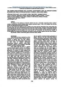
ond half of the last century (Ortúzar and Willumsen 2001; Pečeliūnas and Prentkovskis 2006; Bonzani 2007; Chen et al. 2007; Dragčević et al. 2007; Prentkovskis et al. 2007 and 2009; Sokolovskij and Pečeliūnas 2007; Sokolovskij et al. 2007; Beljatynskij et al. 2009; Junevičius and Bogdevičius 2009; Liu et al. 2009; Vansauskas and Bogdevičius 2009; Viba et al. 2009; Prentkovskis et al. 2010a and 2010b, etc.). This concerns the implementation, analysis and efficiency of safety systems and analysis as well as the simulation of car accidents (Лукошявичене 1988; Иларионов 1989; Lukoševičienė 2001; Sokolovskij et al. 2007; Liu et al. 2009; Viba et al. 2009; Prentkovskis et al. 2010b, etc.). When analyzing the accidents that occurred on the roads of Lithuania, attention was focused on the most frequent type of those − collisions with pedestrians. This allowed to draw both long-term and short-term forecasts for the dynamics of car accidents, to develop a mathematical model of car movement in an accident situation (Lukoševičienė 2001) and to carry out the analysis of calculation methods applied in order to assess the accuracy of the results of studied road traffic accidents (Nagurnas et al. 2007 and 2008). It seems that the number of accidents should depend on both environmental and human factors. However, the analysis of accidents shows that the main cause of road accidents is the latter factor. Among other potential factors, it is worth mentioning the influence of sleepiness and time interval from awakening which has been recently studied (Akerstedt et al. 2008). It is well known that the reaction time of drivers depends on the age and driving experience (Lukoševičienė 2001). This reflects the influence of driver’s experience on the dynamics of road traffic accidents. As a result, the authors have raised a hypothesis that the number of road traffic accidents depends on two components – experience and physical as well as mental condition. To verify this hypothesis, the mathematical simulation of the dependence of road accidents on driving experience has been performed. 2.1. Data Analysis We have analyzed the dependence of the number of accidents on driving experience (Accident Accident Statistics in Lithuania 2010) (see Fig. 1). In order to generate a mathematical approximation, the analyzed data must be properly prepared. For this purpose: – the number of accidents that occurred during the first year (340 accidents) must be assigned to time t = 0.5; – the total number of accidents, i. e. 20, in which the drivers having driving experience of more than 40 years are involved, must be simply eliminated. Later, special analysis is carried out, i.e. the extent to which these assumptions change the generated approximation is verified. It should be noted that the list of accidents contains only data registered by traffic police. We agree that re-

300 Number of motor accidents

238

250 200 150 100 50 0

0

10

20 Driving experience, years

30

40

Fig. 1. The dependence of the number of road traffic accidents on driving experience

quirements for a report on all motor traffic accidents to the police are reasonable. First, this would allow more comprehensive and in-depth analysis. On the other hand, the results of such analysis would be more reliable. 2.2. The Main Trend By using data given in Fig. 1, the assumptions generated above and a certain mathematical package we are able to generate an approximation of these data. The authors have used software package ‘Mathematica’ (license: L2990-7548). Exponential approximation N(t)=ae-bt+c is generated when: a = 307.3, b = 0.1072, c = 14.62.

(2.1)

Parameter a is equal to the initial number of accidents; parameter b may be referred to as the accident rate constant which indicates the relative reduction of the number of accidents per year and determines the rate of changes in the number of accidents with respect to time; parameter c is an asymptotic value which is equal to the number of accidents when driving experience exceeds 40 years. The correlation intervals of parameters a, b and c are as follows: 282.5 < a < 332.1;  0.08549 < b < 0.1289; 0.09 < c < 29.33, 

(2.2)

i .e. halves of the correlation intervals of these parameters are often associated with absolute errors and are respectively equal to ∆a ≈ 24.8; ∆b  ≈ 0.0217; ∆c ≈ 14.6. The approximation curve (trend) with parameters (2.1) and the correlation interval are presented in Fig. 2. The ‘Mathematica’ package allows not only obtaining approximation parameters indicated in formula (2.1), but also assesses the efficiency of the approximation. The efficiency of a mathematical approximation is expressed by a correlation matrix the correlation coefficient of which is equal to 0.814. Parameter 14.6 ≈ 15 may be used to assess the inaccuracy of data, since when t >> 40, the number of accidents should reduce to zero (very old people do not

Transport, 2010, 25(3): 237–243

239

300

N(t) = ae–bt + c

Number of motor accidents

250 200 150 100 50 0

0

10

20

30

40

Fig. 2. The dependence of the number of road traffic accidents on driving experience approximated by the exponential function and correlation interval

drive). On the other hand, a half of the correlation interval of parameter c (2.2) and the related correlation interval show it is approximately equal to the value of parameter c itself. Also, when parameter a is reduced by 10%, the total number of accidents decreases by 36.8%, and in case of reducing parameter b by 10%, the total number of accidents decreases by 17.8%, i.e. their ratio is equal to 2.07. This means that the reduction of the number of accidents during the first driving year is more efficient almost two times than the reduction of accident rate constant b indicating a relative reduction in the number of accidents per year. 2.3. Analysis of Deviations of Real Accidents from the Approximation Curve It follows from Fig. 2 that the approximation curve correctly reflects the downtrend in the number of road traffic accidents. In this subsection, we will analyze the deviations of the number of real accidents from the obtained approximation curve. The approximation formula allows finding the number of predicted accidents at any time. For instance, according to the approximation curve, the drivers with 10 years of driving experience cause 119.8  ≈  120 road accidents on average and the number of real accidents which follows from the data given in Fig. 1 is 142 accidents. This shows that deviation is the difference between the number of real accidents, i.e. 142 and the approximation value, i.e. 120 and is equal to 22 accidents in this case. The data compiled in accordance with this principle are given in Fig. 3 in which the deviations of real values from the approximated ones when driving experience is less than 40 years are reflected.

Table 1. Values of parameters, N20, ω, φ of approximating harmonic function Interval, years

N20

ω

φ

I (0−15)

50.0

0.6

1.2

II (15−40)

6.80

1.21

4.86

2.4. Comments on the Generated Approximations Let us specify the extent to which the assumptions generated in the beginning of this section change parameters a, b, and c of approximation curve ae −bt + c . To this end, a new approximation procedure shall be performed with the changed initial data. If we do not eliminate the last value (the number of accidents caused by drivers with driving experience exceeding 40 years, i. e. 20 accidents), we will obtain the following parameter values: a = 307.3; b = 0.1073; c = 14.74

0

10

20 30 Driving experience, years

Fig. 3. The dependence of the deviations of road traffic accidents on driving experience approximated by harmonic functions and correlation intervals

40

(2.3)

and their correlation intervals: 282.9 < a < 331.7; 0.08635 < b < 0.1283; 0.84 < c < 28.63.

Deviations

50 25 0 –25 –50

The first important conclusion based on the given deviation diagram is that deviations produce periodic vibrations. It is worth noticing that minimum deviation is  – 1.04 when driving experience is 35 years and maximum deviation is 49.4 when driving experience is 11 years. The second important conclusion based on Fig. 3 is that two maximums are evident in case the most frequent causers of road traffic accidents are drivers having 2−3 years of driving experience and those driving for 11−12 years. If the first maximum is well known to everyone, the authors believe that the second one when driving experience reaches 11−12 years is noteworthy. To analyze deviations (Fig. 3), it is appropriate to divide the whole time interval of driving experience into two intervals – less than 15 years and more than 15 years. Deviations when driving experience is less than 15 years form a periodic curve the period of which is approximately 10 years and the amplitude of vibrations from the accidents consists of approximately 50 accidents. When driving experience exceeds the period of 15 years (i.e. in the second interval), the periodicity of accidents decreases to 5 years and the value of amplitude vibration reduces to 15 accidents. Fig. 3 reflects the approximation of deviations of road accidents by harmonic functions the parameter values of which are given in Table 1.

(2.4)

It is evident that the obtained values of parameters a, b and c (2.3) and correlation intervals (2.4) insignificantly differ from respective values (2.1) and (2.2). This is also confirmed by the maximum value of the correlation matrix, i. e. 0.805, obtained with parameters (2.2).

240

P. Miškinis, V. Valuntaitė. Mathematical simulation of the correlation between the frequency of road traffic...

It may be proved that a change of the initial value (340 accidents) when t = 0.4, or t = 0.6 change the values of parameters a, b and c and their correlation intervals even less than in expressions (2.3) and (2.4). Thus, we are sure that the assumptions generated in the beginning of this section are correct. Another question arising when generating any approximation is the choice of the type of the approximation curve. Indeed, why have the authors used an exponential rather than, for instance, a logarithmic approximation? Logarithmic approximation −a ln t + b has at least two advantages: it may be generated with only two parameters: a = 79.67; (73.26 < a < 86.07); b = 300.1; (281.8 < b < 318.4); moreover, the maximum value of the correlation matrix is even 0.94. This shows that the correlation between the logarithmic curve and given data is better than in the case of an exponential approximation. However, the logarithmic approximation has three significant disadvantages: – it follows from the logarithmic approximation that the initial number of accidents is equal to infinity; – there is such driving experience t when the number of road traffic accidents turns to a negative number; – when driving experience highly exceeds 40 years, the number of accidents is negative and infinite. The authors suggest that the abovementioned disadvantages of the logarithmic approximation prevail over its positive characteristics mentioned above. When generating a general approximation, several important principles should be followed: – an absolutely clear and mathematically strict formulation of a task; – the optimal ratio between the elements of the correlation matrix and the characteristics of general data. The first principle determines the type of and the interval in which an approximation is generated etc. For instance, if we are interested in the number of road traffic accidents caused by drivers with driving experience of 1.5 years, we have to perform data interpolation of the initial diagram between values t = 1 and t = 2. This may be power, polynomial or other interpolation. However, if we are interested in the common dependence of road traffic accidents on driving experience in interval [0; 40], an interpolation is not appropriate in this case and other methods should be applied. By applying the second principle, we will come to the conclusion that the approximation curve containing an optimal ratio between the elements of the correlation matrix and conditions for general data would give the value as close to unity as possible for the maximum element of the correlation matrix on the one hand and would be in compliance with the general limits of the initial data, additional conditions or characteristics on the other. For instance, a polynomial or spline approximation is not appropriate in our case because it has no physical meaning. A number of approximation types should

be eliminated due to poor asymptotic characteristics and the like. 3. The Mathematical Model of Accidents The main assumption of the mathematical model for accidents is the statement that the total number of accidents caused by drivers with driving experience t consists of two members: N = (t ) N1 (t ) + N 2 (t ) ,

(3.1)

where: N1 is the number of accidents influenced by driving experience and N 2 is the number of accidents influenced by the physical and emotional condition of drivers. This statement is substantiated by the mathematical analysis of the total number of accidents carried out in the second section. It follows from the second section that the total number of accidents can be expressed as in (3.1), however, the dependency of function N = N(t) and the equation the solution to which is worked out still remain unclear. The purpose of this section is to find a differential equation and its initial conditions describing the total number of accidents N (t ) . It follows from the approximation characteristics of physical and emotional conditions that it is convenient to represent the whole interval of time [0; 40] as the conjunction of two intervals: [0; 40] = [0; 15] ≈ [15; 40]. This means that it is indeed appropriate to develop two models − each model in its interval. The number of accidents that depend on the experience of drivers N1 (t ) may be quite well approximated by exponential function ae −bt + c having parameters (2.1) and correlation intervals (2.2). The damped exponential function is a typical quenching process defined by the first-order differential equation: dN1 (t ) / dt = − b N1 (t ) ,

(3.2)

where: the value of parameter b is equal to the value in the second section (accident rate constant which indicates relative reduction in the number of accidents per year and determines the rate of changing the number of accidents with respect to time) and N10 is the initial number of accidents. It is quite evident that a solution to this equation is damped exponential function: N1 (t ) = N10 e −bt .

(3.3)

The results provided in the second section show that the accident number that depends on the physical and emotional condition of drivers is a periodic function. From all possible types of periodic functions, we will use harmonic functions the differential equation of which is as follows: d 2 N 2 (t ) / dt 2 = −ω2 N 2 (t ) ,

(3.4)

where: ω is the angular frequency of the periodic process.

Transport, 2010, 25(3): 237–243

241

It is not difficult to make sure that function: (3.5)

where: N20 is the initial value of vibrations and φ − the initial phase which is a solution to harmonic vibration equation (3.4). In our opinion, the shift of physical and emotional conditions is more complicated than a harmonic function; however, we will use harmonic functions as the simplest periodic ones the characteristics of which are well known. It would be appropriate to use the functions that are more complicated than harmonic ones; however, in order to determine the exact difference between harmonic and non-harmonic functions, a larger base of statistical data is necessary. Having in mind that the total number of accidents N (t ) is the sum of two trends (3.1), using differential equations (3.2) and (3.4) and defining these trends, we obtain that the function defining the total number of accidents N (t ) satisfies the differential equation: d 2 N / dt 2 + bdN / dt + f (t ) = 0; N (1) = N 0 ; N ′(1) = N 0′ ,

Table 2. Values of approximating parameters N0, N 0′ , b, N20, ω, φ in the corresponding expressions

I (0−15)

II (15−40)

N0

307.3

b

0.1072

N 0′

32.95

N20

63

3

ω

0.5

0.9

φ

–2.3

–2.6

350

(3.6)

where: f (t ) is the known function and N 0 and N 0′ are initial conditions. It is worth noting at least two significant characteristics of this equation: – it is a simple differential equation rather than the equation involving partial derivatives; – this differential equation is linear. These characteristics allow obtaining an analytical solution to differential equation (3.6):

Intervals, years

Parameters

300 Number of accidents

,

A summary of parameter b, function f(t) and initial conditions is given in Table 2. In Fig. 4, one can find the approximated results of the offered model (3.6).

ACM[0,15] = 0.987 ACM[15,40] = 0.965

250 200 150 100 50 0

0

10

20 30 Driving experiance, years

40

Fig. 4. An approximation of the dependence of road traffic accidents on driving experience applying the proposed mathematical model

(3.7)

The second-order simple differential equation including initial conditions (3.6) and its analytical solution (3.7) constitutes the mathematical model of the dependence of the total number of road traffic accidents on driving experience. In order to define this model in terms of quantity, parameter b, function f(t) and initial conditions should be specified in more detail. We will find initial conditions N 0 and N 0′ from the approximation exponential function given in the second section showing that N 0 = 307.3 . Considering that parameter b shows the reduction of accidents per year, we will determine the value as bN 0 . From b = 0.1072 and N10 = 307.3, we obtain that = N 0′ b= N 0 0.1072×307.33 = 32.95. Functions f(t) are different in both intervals: = f I 63cos(0.5t − 2.3); = f II 3cos(0.9t − 2.6).

(3.8)

The maximum elements of the asymptotic correlation matrix (ACM) have been given in the respective intervals of driving experience (less than 15 years and from 15 to 40 years). The areas of an abnormally high accident rate, i.e. 2−3 years and 11−12 years, have been distinguished 4. The Main Characteristics of the Model It should be noted that a differential equation of the main model (3.6) may be replaced by the first-order differential equation after changing the variables in terms of mathematics. Only one initial condition is necessary for its solution and it seems that such a model would be simpler. However, we will not get an advantage in terms of initial conditions: in order to compare the number of real accidents (Fig. 1), the integration of the solution to the differential equation should be performed and the necessary integration constant should be predefined. In physics, the second-order differential equation: d 2 N / dt 2 + bdN / dt + ω2 N = f (t )

(4.1)

P. Miškinis, V. Valuntaitė. Mathematical simulation of the correlation between the frequency of road traffic...

242

is referred to as the equation of damped forced vibrations in which parameter b is referred to as a damped coefficient, ω is the frequency of free vibrations and F (t )  – forced external force. When forced external force is a harmonic function, the solution to this equation is well known. By analogy with damped vibrations in physics, two important identities correlating with parameters of the offered model may be formulated in our case: N m0 =

2 fm 0 ωm b2 + 2ω2m

b ; tg ϕ 1 = , ω

(4.2)

where: fm 0 (m =I, II) are the values of the amplitude of functions f I , f II (3.8) and their frequencies and ωm is phase difference between function f(t) and solution N(t). It follows from formula (3.10) that by inserting the respective values from formula (3.8) into this expression, we will obtain that N m 0 ≈ fm 0 and ϕ 1 ≈ 0. This means that amplitude deviations from the main tendency (trend) are equal to the amplitude values of function fm(t) and phase difference between these functions is negligible. Another consequence resulting from this analogy in physics is the fact that if the initial number of accidents is reduced, then the number of all accidents not only decreases but also may completely disappear. Since the number of accidents may not be negative, if the initial number of accidents is reduced to ~50, we will obtain that, for instance, the number of accidents in the group of drivers having driving experience of 11−13 years will entirely disappear which additionally reduces the total number of accidents. It is probably impossible to generate a uniform approximation within the limits of a linear model in the whole interval [0; 40] because periodic functions f I , f II in intervals [0; 15] and [15; 40] (this follows from expression (3.9) differ not only in the amplitude but also in the period. Continuous transition without division into two intervals is probably possible in the approximation of a non-linear model and requires more detailed information. Finally, we will verify the model by means of the functions approximating five parameters similar to the eigenfunctions of the proposed mathematical model. Table 3. Values of approximating parameters N10, b, N20, ω, φ Parameters N10

Intervals, years I (0−15) II (15−40) 337.1

b

0.1061

second (15–40 years). Such values of the elements of the asymptotic correlation matrix could be considered as very good (Ortúzar and Willumsen 2001). 5. Conclusions We would like to emphasize that this article is not mere processing of statistical data which provides a mathematical model allowing forecasting the situation in case of changing one or another parameter of the model. We will remind that our ultimate purpose is decreasing the total number of road traffic accidents, i.e. the possibly smallest data distribution area (Fig. 1) rather than the development of the model. The properties of the proposed mathematical model are as follows: – it is reasonable to represent the total number of accidents as a sum of two processes: experience + physical and emotional condition; – separate mathematical models proposed for each interval indicating the experience of drivers: less than 15 years and from 15 to 40 years; – the number of accidents exponentially decreases with an increase in driving experience: N1 (t ) = 307.3exp( − 0.1072 t ) − 14.62 ; – the number of accidents that depend on the physical and emotional conditions of drivers N 2 (t ) is a periodic rather than a harmonic function and has the following characteristics: a) two-time intervals [0; 15] ∪ [15; 40] and two maximums – 2/3 years and 11−12 years. These time intervals correlate with the dependence of divorces on the length of marriage; however, quantitative results require more in-depth analysis; – the maximum elements of the asymptotic correlation matrix have the value of ~0.8 and the coefficient of such correlation is regarded as quite high also in the statistical analysis of transport systems (Ortúzar and Willumsen 2001); – if the initial number of accidents N0 is reduced in the group of drivers having experience of 11−13 years, the number of accidents will totally disappear. Our goal is not to comprehensively and explicitly answer the question of how to reduce the total number of fatalities in Lithuania. We have only analysed the consequences of the available statistical data for the dependence of the number of accidents on driving experience and believe that the results of this analysis deserve consideration. Acknowledgment

29.72

2.953

ω

0.7826

0.8858

We sincerely thank the reviewers for benevolent attention to our manuscript and useful remarks made.

φ

–2.343

–2.568

References

N20

Let us note that the values of the asymptotic correlation matrix of this verification are 0.84 for the first driving experience interval (0–15 years) and 0.97 for the

Accident Statistics in Lithuania. 2010. Lithuanian Road Police Office. Available from Internet: . Akerstedt, T.; Connor, J.; Gray, A.; Kecklund, G. 2008. Predicting road crashes from a mathematical model of alertness

Transport, 2010, 25(3): 237–243 regulation − the sleep/wake predictor, Accident Analysis and Prevention 40(4): 1480–1485. doi:10.1016/j.aap.2008.03.016 Beljatynskij, A.; Kuzhel, N.; Prentkovskis, O.; Bakulich, O.; Klimenko, I. 2009. The criteria describing the need for highway reconstruction based on the theory of traffic flows and repay time, Transport 24(4): 308–317. doi:10.3846/1648-4142.2009.24.308-317 Bonzani, I. 2007. Hyperbolicity analysis of a class of dynamical systems modeling traffic flow, Applied Mathematics Letters 20(8): 933–937. doi:10.1016/j.aml.2006.06.022 Chen, T.; Chirwa, E. C.; Mao, M.; Latchford, J. 2007. Rollover far side roof strength test and simulation, International Journal of Crashworthiness 12(1): 29–39. doi:10.1533/ijcr.2006.0156 Dragčević, V.; Korlaet, Ž.; Stančerić, I. 2008. Methods for setting road vehicle movement trajectories, The Baltic Journal of Road and Bridge Engineering 3(2): 57–64. doi:10.3846/1822-427X.2008.3.57-64 Elvik, R.; Mysen, A. B.; Vaa, T. 1997. Trafikksikkerhetshandbok [Handbook of Traffic Safety]. Transportokonomisk institutt [Institute of Transport Economic], 3rd edition. Oslo. Junevičius, R.; Bogdevičius, M. 2009. Mathematical modelling of network traffic flow, Transport 24(4): 333–338. doi:10.3846/1648-4142.2009.24.333-338 Liu, Z.-Q; Wang, P.; Zhang J.-H. 2009. Study on reproduction of car-to-car oblique crash based on reverse-reasoning calculation, Journal of Highway and Transportation Research and Development 26(1): 144–148. Lukoševičienė, O. 2001. Autoįvykių analizė ir modeliavimas: monografija [The road accident analysis and simulation: Monograph]. Vilnius: Technika. 244 p. (in Lithuanian). Nagurnas, S.; Mitunevičius, V.; Unarski, J.; Wach, W. 2007. Evaluation of veracity of car braking parameters used for the analysis of road accidents, Transport 22(4): 307–311. Nagurnas, S.; Mickūnaitis, V.; Pečeliūnas, R.; Vestertas, A. 2008. Analysis of calculation methods used for accuracy evaluation of the results of road accident examination, Transport 23(2): 156−160. doi:10.3846/1648-4142.2008.23.156-160 Ortúzar, J. de D.; Willumsen, L. G. 2001. Modelling Transport. 3rd edition. Wiley. 514 p. Pečeliūnas, R.; Prentkovskis, O. 2006. Influence of shock-absorber parameters on vehicle vibrations during braking, Solid State Phenomena 113: 235–240. doi:10.4028/www.scientific.net/SSP.113.235 Prentkovskis, O.; Prentkovskienė, R.; Lukoševičienė, O. 2007. Investigation of potential deformations developed by elements of transport and pedestrian traffic restricting gates during motor vehicle–gate interaction, Transport 22(3): 229–235. Prentkovskis, O.; Beljatynskij, A.; Prentkovskienė, R.; Dyakov, I.; Dabulevičienė, L. 2009. A study of the deflections of metal road guardrail elements, Transport 24(3): 225–233. doi:10.3846/1648-4142.2009.24.225-233 Prentkovskis, O.; Beljatynskij, A.; Juodvalkienė, E.; Prentkovskienė, R. 2010a. A Study of the deflections of metal road guardrail post, The Baltic Journal of Road and Bridge Engineering 5(2): 104–109. doi:10.3846/bjrbe.2010.15 Prentkovskis, O.; Sokolovskij, E.; Bartulis, V. 2010b. Investigating traffic accidents: a collision of two motor vehicles, Transport 25(2): 105–115. doi:10.3846/transport.2010.14 Sokolovskij, E.; Pečeliūnas, R. 2007. The influence of road surface on an automobile’s braking characteristics, Strojniski Vestnik – Journal of Mechanical Engineering 53(4): 216–223.

243 Sokolovskij, E.; Prentkovskis, O.; Pečeliūnas, R.; KinderytėPoškienė, J. 2007. Investigation of automobile wheel impact on the road border, The Baltic Journal of Road and Bridge Engineering 2(3): 119–123. Šliupas, T. 2009. The impact of road parameters and the surrounding area on traffic accidents, Transport 24(1): 42–47. doi:10.3846/1648-4142.2009.24.42-47 Vansauskas, V.; Bogdevičius, M. 2009. Investigation into the stability of driving an automobile on the road pavement with ruts, Transport 24(2): 170–179. doi:10.3846/1648-4142.2009.24.170-179 Viba, J.; Liberts, G.; Gonca, V. 2009. Car rollover collision with pit corner, Transport 24(1): 76–82. doi:10.3846/1648-4142.2009.24.76-82 Иларионов, В. А. 1989. Экспертиза дорожно-транспортных происшествий [Ilarionov, V. A. Examination of Road Traffic Accidents]. Moсква: Транспорт. 254 с. (in Russian). Лукошявичене, О. В. 1988. Моделирование дорожнотранспортных происшествий [Lukoševičienė, O. Simulation of traffic accidents]. Москва: Транспорт. 96 с. (in Russian).