In a recent issue of The American Statistician, there was a discussion on the desirability of teaching a rst statistics course from a Bayesian viewpoint. To see ...
MATLAB as an Environment for Bayesian Computation Jim Albert1
Bowling Green State University July 1997
Address for correspondence: Department of Mathematics and Statistics, Bowling Green State University, Bowling Green, OH 43403, USA. 1
Abstract The current status of Bayesian software is reviewed. The motivation for the development of Bayesian software is described and the software is categorized by the type of user (student, practitioner, and researcher). The use of the software package MATLAB is illustrated for the di�erent types of Bayesian software. The use of a MATLAB graphical user interface (gui) is demonstrated for the introduction of proportion inference using a discrete prior. A second gui is used to illustrate the use of a MCMC algorithm in logistic modeling with a data augmented prior. The use of MATLAB as a programming environment for the development of MCMC algorithms is discussed, and a MCMC program for tting a random e�ects model is outlined.
1 An overview of Bayesian software 1.1 What's available?
In a recent issue of The American Statistician, there was a discussion on the desirability of teaching a rst statistics course from a Bayesian viewpoint. To see which statistical methods are actually used in practice, Moore (1997) surveyed a large number of published articles in applied statistics disciplines. He noted that very few articles actually employed Bayesian methods. Although Bayesian articles are widely prevalent in the major journals in the research of statistics (look at a recent issue of the Journal of the American Statistical Association), it is clear at this time that Bayesian thinking hasn't generally reached the population of applied statisticians. Why aren't Bayesian methods more popular? There are many reasons suggested for its lack of popularity, including the lack of Bayesian courses in graduate statistics courses, a general concern over the choice of a prior distribution, and the disagreement among Bayesians about a reasonable \default" posterior analysis for many problems. (Moore (1997) discusses these reasons in his teaching article.) One major stumbling point for the popularity of Bayesian analyses, pointed out by Berry (1997), is the lack of general software to perform Bayesian analyses. Most current textbooks in applied statistics link the discussion of methodology with available statistical software. In fact, one can discover the popular statistical methods by reading a statistical software guide for a popular package such as SAS, SPSS, or Minitab. It is clear that Bayesian methods will not become more popular among practitioners until much more Bayesian software is available. Carlin and Louis (1996) provide a comprehensive listing of Bayesian software that is currently available. It is notable that most of the Bayesian programs listed in this book are not commercially produced. Most of the program developers come from academia and the software represents an implementation of recent published research articles. Since little Bayesian commercial software is currently available, it appears that there is a need for a general discussion about how a Bayesian software enterprise should develop. This discussion should address the following issues:
� What is the reason for Bayesian software? From the practitioners' viewpoint, what is gained from the methods implemented in Bayesian software that is not available from traditional methods and software?
� How should Bayesian software di�er from software to perform traditional statistical 1
analyses? Will the Bayesian software just add a prior to a classical software package?
� Can Bayesian methods be added to a currently popular statistics software package?
Is it possible to have a Bayesian SAS? Is this something that we (as Bayesians) would like to see?
� More generally, are there good high-level mathematical or statistical computing envi-
ronments for the development of Bayesian software? Examples of such environments are statistical systems such as S-Plus, and mathematics systems such as Mathematica, Maple, and MATLAB.
1.2 Why Bayes? For a commercial Bayesian software package to become popular, the developers will need to reach an audience far wider than the current group of Bayesian statisticians. A traditional applied statistician will be interested in Bayesian software and the associated methods only if there is something to be gained by a Bayesian approach. Berger (1985) makes persuasive arguments in favor of a Bayesian viewpoint towards inference. He states that important prior information can be available, uncertainty should be expressed probabilistically, there are advantages to a conditional viewpoint towards inference, and Bayes rules are coherent. Are any of these arguments relevant when a marketing rm wishes to sell Bayesian software? Statisticians embrace the Bayesian viewpoint for di�erent reasons, depending on the particular application of interest. This article will focus on two speci c areas: the teaching of statistical inference and the tting and checking of generalized linear models. What are the advantages of a Bayesian perspective for these two speci c applications?
Teaching There are good reasons for introducing statistical inference from a Bayesian perspective. (See Albert (1997) and Berry (1997).)
� The Bayesian paradigm is a natural way of implementing the scienti c method where
the prior represents your initial belief about a model, you collect relevant data, and the posterior represents your updated beliefs after seeing the data.
� If uncertainty about models is expressed using subjective probability, then Bayes' rule is the only recipe one needs to perform inferences from data. 2
� Bayesian inferential statements are easier to understand than traditional inferential
statements based on repeated sampling. The probability that a parameter falls inside a computed interval is equal to .95. Likewise, in contrast with traditional testing procedures, it is meaningful to talk about the probability that a statistical hypothesis is true.
� By the conditionality principle, the only data relevant to performing inference is the actual data that is observed. One can ignore other data outcomes in the sample space that are not observed.
� Prediction problems are essentially no more di�cult than parameter estimation problems. Parameters and future observables are both unknown quantities that are modeled subjectively.
Generalized linear models Generalized linear models (glm's) have become increasingly popular since their introduction by Nelder and Wedderburn (1972). They have provided a general framework for modeling a response variable from the exponential family. Examples of glm's include linear regression with normal errors, logistic regression for binary data, log-linear modeling for Poisson data, and survival model for Weibull and gamma data. It is relatively easy to write software for tting glm's since there is one general algorithm for nding maximum likelihood estimates for the regression coe�cients. The popularity of glm's is partially due to the emergence of the associated software package GLIM for tting and checking these models. What are the advantages of a Bayesian perspective to glm's?
� The classical analysis of a glm is based on the asymptotic normal approximation to the
sampling distribution of the mle and on the asymptotic chi-squared approximation to the deviance statistic. A Bayesian analysis with a noninformative prior allows one to perform exact inference on the likelihood function. This may be desirable in small or sparse data situations where the accuracy of the classical distribution approximations can be poor.
� A Bayesian analysis allows one to input prior information. This is particular helpful in the case where little data are observed and subjective input can play an important role in the nal inference. We will discuss later on how one can input prior beliefs into a glm. 3
� Bayesian hierarchical modeling is especially useful for glm's when it is desirable to combine related groups of data.
1.3 What is the target audience? The development of any Bayesian software package must have a clear view of the intended audience. If one categorizes all Bayesian software by means of the type of user, then there are the following three broad categories of software.
� Teaching Bayes This Bayesian software would provide an introduction to prior elici-
tation, inference, and prediction for the standard sampling models covered in the rst statistics course. The intended audience would be undergraduate and graduate students in students and applied statisticians who are being introduced to the Bayesian viewpoint.
� Modeling Bayes This software is application speci c. It would provide Bayesian
methods for a speci c application such as normal regression, time series, generalized linear models, or expert systems. The target audience for say, Bayesian time series software, would be those statisticians in academia or industry who routinely analyze time series data.
� Research Bayes There is a general need for software to meet the needs of people who are developing new Bayesian models and tting procedures. These researchers typically write their own computer programs to implement their procedures and there is a need for a package of computer subroutines, such as a simulation package, to make it easier to program.
1.4 MATLAB This article will illustrate di�erent types of Bayesian software using the MATLAB programming language. What is MATLAB? It is an interactive high-level language for integrating computation, visualization, and programming. It was originally written to provide an easy access to matrix software developed by the LINPACK and EISPACK projects. The basic data element in MATLAB is a matrix. One performs calculations by entering calculatortype instructions in the Command Window. Alternatively, one can execute sets of commands by means of scripts called M- les and functions. MATLAB has extensive facilities for displaying vectors and matrices as graphs. 4
MATLAB is especially popular in the elds of mathematics, engineering, and science. Many application-speci c collection of programs, called toolboxes, have been developed over the years. Areas in which toolboxes are available include signal processing, control systems, neural networks, wavelets, and simulation. MATLAB has the ability to interact with C and Fortran programs. The new version of MATLAB allows to one to build complete Graphical User Interfaces for applications. MATLAB has the potential to become an excellent interactive computing environment for statistics. However, it currently lacks the large number of developed statistical applications that are available in the interactive system S-Plus. A MATLAB statistics toolbox has been recently written and is being expanded. This toolbox contains functions to compute and simulate from all of the common probability distributions. In addition, it contains routines to compute a variety of descriptive statistics and programs for linear and nonlinear modeling, design of experiments, statistical process control, and principal compnents analysis. The aim of this article is to illustrate the potential of MATLAB as a general computing environment for the three broad types of Bayesian software described above. Section 2 rst considers the development of Bayesian software for teaching purposes. The student audience is likely not very familiar with mathematics or statistics software and it may be unwise to devote a signi cant portion of the course for learning a new programming environment. However, MATLAB can be used to develop a user-friendly graphical user interface (gui) for basic Bayes computations. The student using this gui needs to know nothing about the MATLAB matrix language to get results. This section illustrates Bayesian inference for a proportion using a discrete prior and indicates how conjugate Bayesian analyses could be programmed in this environment. Section 3 considers an example of the application-oriented type of Bayesian software | Bayesian logistic regression. We illustrate the use of a MATLAB gui which allows for the input of the prior distribution, explores the posterior distribution of the regression parameter by means of a Markov chain Monte Carlo (MCMC) algorithm, and gives various graphical and numerical summaries of the simulated posterior distribution. Section 4 discusses the development of a MATLAB toolbox to aid the researcher of Bayesian simulation-based methodology. We give an example of using MATLAB to program a MCMC algorithm using an example problem described in the BUGS example manual.
5
2 A teaching Bayes toolbox 2.1 Discrete priors
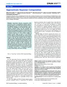
An attractive method of introducing the Bayesian viewpoint is through the use of discrete priors. We illustrate the use of this type of prior in inference about a population proportion. Suppose one observes independent observations X1 ; :::; Xn from a Bernoulli distribution with probability of success p. The parameter p can be interpreted as the proportion of successes in a population divided into successes and failures. If g(p) denotes the prior density for p, P then the posterior density is given by g(pjdata) / g(p)ps (1 ? p)f , where s = ni=1 xi is the observed number of successes and f = n ? s the number of failures. A construction of a subjective prior distribution for p can be introduced by the use of a discrete prior density g(p). Let p1 ; :::; pk denote k plausible values of the proportion. One can build a prior on this set of values by considering relative likelihoods. One could begin by assigning a mass of 100 to the most likely proportion value, 50 to values of p which are half as likely as the modal value, 10 to values which are 1/10 as likely as the modal value, and so on. This assessment process can be easier than directing specifying probabilities for the individual values. We illustrate the use of a MATLAB gui to give the student experience in the construction of a discrete prior and in the interpretation of the resulting posterior distribution. The students runs a MATLAB m- le which generates the gui displayed in Figure 1. A default uniform prior on the proportion values p = 0; :1; :::; 1 is displayed at the top of the window. A prior is constructed in two steps: 1. An equally spaced grid of proportion values is created by pressing the \De ne Prior Grid" button. When this button is pressed, the user is asked to input the smallest proportion value, the largest proportion value, and the number of values. 2. A uniform set of probabilities is shown in the top graph for the grid de ned by the user. One can then adjust these prior probabilities graphically by clicking the mouse on the graph. One changes the height of a particular bar by clicking the mouse below or above the top of the bar. After some experimentation, the user can construct a prior distribution which approximates his or her prior beliefs. As an illustration of this assessment process, suppose that a user if interested in learning about the proportion of defective components in a shipment. From previous experience, she believes that proportion values between .01 and .20 are possible and smaller proportion 6
values are most probable. She chooses a grid of 20 equally spaced values between .01 and .20. By adjusting the bar heights, she constructs a distribution (top display of Figure 2) which roughly ts her prior beliefs. After this prior is constructed, one enters in data and updates the probabilities by means of two buttons in the middle of the window. The \Get Data" button brings up a dialog box where one enters the numbers of successes and failures s and f . The \Update" button will compute the posterior probabilities. The graph of the posterior distribution is shown in the bottom display. The actual table of probabilities is displayed in a list box. Basic summaries of the posterior distribution (the mean, standard deviation, and 90% probability interval) are displayed in a box next to the probability table. In our example, suppose that 20 components are inspected and 2 are found defective (so s = 2 and f = 18). The user enters the data. The posterior probabilities are shown in the lower display of Figure 2. This is a relatively simple program, but its ease of use should encourage the student to experiment with di�erent priors and see the e�ect of di�erent datasets. Does it matter if one uses a uniform prior or a subjective nonuniform prior? What is the e�ect of choosing a ne grid of proportion values? How does the posterior distribution change one increases the sample size n from 20 to 100? This device is also useful for motivating a continuous prior for a proportion. If one uses a very ne grid, then the prior and posterior densities will look like smooth curves. By inspecting the posterior probability table, one notes that it is not very meaningful to discuss the probability that a proportion is equal to a speci c value (it is close to 0). However, it is meaningful to discuss probabilities of intervals. This discrete approach to prior modeling can be used for a variety of parameter inference problems. Albert (1995) illustrates this approach for inference about a normal mean with known variance, a Possion mean, an exponential mean, a hypergeometric proportion, and the unknown upper bound of a discrete uniform distribution. (A collection of MINITAB macros to implement this discrete approach to modeling is described in Albert, 1996b.) The gui interface for this class of models would remain the same as described above. One would just need to add a submenu where one inputs the sampling distribution (binomial, normal, Poisson, exponential, etc.).
7
PRIOR DISTRIBUTION
prob
0.15 0.1 0.05 0
0
0.2
0.4
0.6
0.8
1
0.8
1
p
POSTERIOR DISTRIBUTION
prob
0.2 0.1 0
0
0.2
0.4
0.6 p
Figure 1: Opening view of a MATLAB gui to perform inference about a binomial proportion using a discrete prior.
8
PRIOR DISTRIBUTION
prob
0.2 0.1 0
0
0.02
0.04
0.06
0.08
0.1
0.12
0.14
0.16
0.18
0.2
0.16
0.18
0.2
p
POSTERIOR DISTRIBUTION
prob
0.1 0.05 0
0
0.02
0.04
0.06
0.08
0.1
0.12
0.14
p
Figure 2: Display of the MATLAB gui after constructing a subjective prior and updating with observed data.
9
2.2 Conjugate priors A second way of introducing Bayesian inference is by the use of conjugate prior distributions. The First Bayes program (O'Hagen, 1994) provides a graphical interface for performing conjugate inference for a number of standard distributions including binomial, Poisson, and normal with known variance, and for normal linear regression. This program allows the use of mixtures of conjugate prior distributions, and provides numerical and graphical summaries of posterior and predictive distributions. A toolbox of MATLAB functions could be written to perform posterior and predictive inference for these conjugate families. In the binomial proportion inference problem, one MATLAB function could take as input the parameter values of the beta prior and the binomial data and output the parameter values of the beta posterior. A second function could output the predictive distribution given the parameters of the beta prior and the future sample size. There are other tools that may be useful in the application of Bayesian conjugate inference. One advantage of the use of conjugate priors is that subjective prior input can be modeled through the hyperparameters of the priors. A number of MATLAB functions could be written to aid in this prior assessment process. For example, a beta prior density can be speci ed by giving two fractiles of the distribution, or by statements about the prediction distribution of a future binomial sample. MATLAB functions could be used to quickly see the relationship between, say, the speci ed fractiles and the resulting beta prior density. In addition, conjugate inference can be used to introduce simulation as a device for representing prior distributions. For example, a beta posterior can be represented by the use of a simulated sample taken from this distribution using the MATLAB betarnd command found in the Statistics Toolbox. Summaries of this beta posterior such as a mean, standard deviation, or percentiles can be easily found by means of the corresponding summaries of the simulated sample.
3 Bayesian tting of generalized linear models Next we consider the development of Bayesian software for regression modeling where the response variable is a member of the exponential family. Suppose, for example, that we observe response proportions y1 ; :::; yN from binomial populations with proportions p1 ; :::; pN and corresponding sample sizes n1 ; :::; nN . Associated with the ith observation, there is a vector of covariates xi , and the proportion pi is linked to the covariates xi by means of the 10
logistic model
log(pi =(1 ? pi )) = xTi :
The likelihood of the regression vector is given by
L( ) = where
YN pn y (1 ? p )n
i=1
i
i i
i
?y ) ;
i (1
i
T pi = 1 +expexp(x(ix T) ) : i
If g( ) is the prior density for , then the posterior density of is proportional to
g( jy) = g( )L( ):
3.1 Choosing a prior Bayesian software should provide a means of constructing the prior density g( ). In this setting it is di�cult to directly assess a prior on the regression parameter since it related in a nonlinear fashion to the probabilities fpi g. Following Bedrick et al (1996), it is probably easier to indirectly specify a prior on by making statements about the mean proportion value E (p) at selected values of the covariates. If the rank of the covariate matrix is k, then one considers the proportions p1 ; :::; pk at k di�erent sets of values at the covariate x. The conditional means prior (CMP) assumes that p1 ; :::; pk are independent with pi distributed Beta(wi mi ; wi (1 ? mi )), where mi is the prior guess at pi and wi is the precision of this guess. The prior on p1 ; :::; pk is proportional to
g(p1 ; :::; pk ) =
Yk pw m ? (1 ? p )w
i=1
i
i
i
1
i
?m )?1 :
i (1
i
Bedrick et al (1996) show that, for the logistic link, this prior on fpi g is equivalent to a prior on that is the same form as the likelihood with \prior observations" f(mi ; wi ; xi )g. (This is called a data augmented prior (DAP).) It is easy to update the posterior density on using this form of prior information. The posterior density is proportional to
g( jy) =
YN pn y (1 ? p )n
i=1
i
i i
i
?y )
i (1
i
Yk pw m (1 ? p )w
j =1
i
i
i
i
?m )
i (1
i
In other words, the posterior on is equivalent to the likelihood of the observed data f(yi ; ni; xig augmented by the \prior data" f(mj ; wj ; xj )g. 11
3.2 Summarizing the posterior density After the prior information is speci ed and the data is observed, the task of the software is to e�ectively summarize the posterior density of the regression vector . One good strategy for this summarization is to rst approximate the posterior density with a normal distribution with matching mode and curvature at the mode. Then this normal distribution can be used to construct a Markov chain Monte Carlo (MCMC) simulation from the exact posterior density. Suppose that the mode and associated variance-covariance matrix of are given by ^ and V respectively. The mode ^ provides a good starting point for the Markov chain simulation. A relatively simple but e�ective MCMC algorithm in this setting is a random walk chain using a multivariate normal proposal density. Let c denote the current value of in the random walk. Then a proposal value p , is given by
p = c + Z; where c is the current simulated value and Z is a multivariate normal random with mean vector 0 and variance-covariance matrix V . The random walk will move to the proposed value p with probability P , where p data) P = min(1; gg(( c jjdata) ): If the random walk is continued for a large number of iterations, then the stream of simulated values of is approximately distributed from the posterior density.
3.3 Analyzing the simulation output Generally, in a MCMC simulation, one has to be concerned with convergence and the size of the simulation sample. Equivalently, does the current string of simulated values approximate the joint posterior density of interest, and, if it does, has a large enough sample been taken to provide good estimates at posterior summaries, such as means and standard deviations? From experience, this type of glm likelihood appears not to have convergence problems. Running one long chain is a suitable strategy in this situation and one can informally check if there is suitable mixing by inspecting a trace graph of the simulated values for components of or for a function f ( ). This trace graph is also helpful in informally checking if the size of the simulated sample is su�ciently large. If the trace plot of any component of shows signi cant drift or instability, then likely the simulation should be rerun with a larger number of iterations. 12
If the display of a number of trace graphs indicates no problems, then summarizing the posterior density is similar to the process of summarizing a large multivariate dataset. A histogram of the simulated values of a function f ( ) is a rough graph of its marginal posterior density. A empirical cdf plot of the simulated values is helpful for understanding the location of f ( ) and for picking out percentiles of interest. After the inspection of some graphs, one may be interested in summarizing a particular marginal posterior density by a mean, a standard deviation, and a probability interval.
3.4 An example We illustrate the use of a MATLAB gui in tting a logistic model using a dataset from Vaisanen and Jarvinen (1977) and analyzed in Ramsey and Schafer (1996). Table 1 presents data collected from an extensive bird study of the Krunnit Islands archipelago. For each of 20 islands, the area in square kilometers, the number of species at risk, and the number of extinctions are given. (An extinction is de ned as a species that was present at the island in 1949 but not present in 1959.) Le pi denote the probability of bird species from island i is extinct. A suggested model is log(pi =(1 ? pi )) = 0 + 1 xi ; where xi is the log of the area of the ith island. Suppose that the researcher has some prior beliefs about the relationship between island size and extinction probability. She believes that the size of island has some e�ect on the probability. For a large island of size log 2 = 7:4 km2 , she guesses that the extinction probability is .1; for a smaller island of size log ?2 = :14 km2 , she thinks that the extinction probability has increased to .2. Both of these guesses are worth about 5 prior observations. This prior information corresponds to a conditional means prior with (m1 ; w1 ; x1 ) = (:1; 5; ?2) and (m2 ; w2 ; x2 ) = (:2; 5; 2). The data is stored as a matrix. This matrix has the general form data = [y n x]
where y is a column vector of observed proportions, n is a column vector of sample sizes, and x is the design matrix including a column of ones for the constant term. Similarly, a data-augmented prior can be stored as the matrix prior = [m w x]
13
Table 1: Data from the Krunnit Islands Study. Island Area (km2 ) Species at Risk Extinctions Ulkokrunni 185.80 75 5 Maakrunni 105.80 67 3 Ristikari 30.70 66 10 Isonkivenlettto 8.50 51 6 Hietakraasukka 4.80 28 3 Kraasukka 4.50 20 4 Lansiletto 4.30 43 8 Pihlajakari 3.60 31 3 Tyni 2.60 28 5 Tasasenletto 1.70 32 6 Raiska 1.20 30 8 Pohjanletto 0.70 20 2 Toro 0.70 31 9 Luusiletto 0.60 16 5 Vatunginletto 0.40 15 7 Vatungnnokka 0.30 33 8 Tiirakari 0.20 40 13 Ristikarenletto 0.07 6 3
14
TRACE PLOT −0.1 −0.15 −0.2 −0.25 −0.3 −0.35 −0.4 −0.45 −0.5 −0.55
0
2000
4000
6000
8000
10000
beta
1
Figure 3: Display of the MATLAB logistic model gui to investigate the convergence of MCMC run to the posterior distribution. where m is the vector of prior means of the probabilities, w are the prior sample sizes corresponding to these prior means, and x is the design matrix at which these prior means are taken. A MATLAB gui which will t a logistic model with prior information is displayed in Figure 3. The user rst loads the data by pushing the \Load Data" button and selecting the stored data le in a dialog box. The prior data matrix can be loaded by pushing the \Load Prior" button. Next, one selects the number of iterations of the MCMC algorithm by means of the pop-up menu. The model is t by pushing the \Run Simulation" button. In the rst run, no prior information was loaded | the default prior will be a at prior on the regression vector . The number of iterations was chosen to be 10,000. The MCMC run took 65 seconds to run on a Pentium 90 machine. This gui encourages graphical exploration of the matrix of simulated values of to assess convergence of the simulation algorithm and to summarize the posterior distribution. To produce a graph, one selects the component of in the \Parameter" pop-up menu, selects the type of graph in a pop-up menu, and then pushes the \Plot" button to produce the display. If one is interested in plots of a function f ( ), then one enters its de nition in the \Function de nition" text eld box in the lower left corner, and then selects \Function" in the parameter pop-up menu. 15
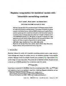
To investigate convergence of the MCMC algorithm, it is helpful to view trace plots of individual components of or a function of interest. Figure 3 shows a trace plot of the regression slope 1 . This plot shows no drift and good mixing. From looking at a number of plots such as this one, it is reasonable to believe that the stored simulated sample is a good representation from the posterior distribution. The program lets one summarize components of or a function f ( ) by means of a histogram, a empirical cdf, and by a mean, a standard deviation, and a 90% probability interval. The numerical summaries of the parameter chosen in the parameter pop-menu menu are found by pushing the \Summaries" button. Suppose, for example, that one is interested in learning about the probability of extinction when the log area of the island is x = ?1. This probability can be expressed as 0 ? 1 ) p = 1 +exp( exp( 0 ? 1 ) : This function is programmed in MATLAB as the inverse logit function ilogit. In the function de nition box, we enter the text ilogit(beta_0 - beta_1)
We then select \function" in the parameter pop-up menu, select \histogram" in the type of graph pop-up menu, and press the buttons \Plot" and \Summaries". The display of the gui is shown in Figure 4. (In this particular run, we used the prior information as described above.) We estimate this probability to be .285 and a 90% interval is (.238, .334). From repeated use of this gui for di�erent choices of the function f , one can e�ectively learn about this logistic t.
4 A Bayesian computational toolbox 4.1 Systems for Bayesian computation
In the last fteen years, there have been a number of attempts to create general systems for Bayesian computation. The Bayes 4 system (Naylor and Smith, 1985) was one of the earlier programs developed. It was designed to summarize an arbitrary posterior distribution using a number of methods including adaptive quadrature (Naylor and Smith, 1982) and a variety of simulation methods. For a particular problem, the logarithm of the posterior distribution would be de ned in a Fortran subroutine, and the user would interactively explore this 16
HISTOGRAM 3500 3000 2500 2000 1500 1000 500 0 0.15
0.2
0.25
0.3 0.35 function
0.4
0.45
0.5
Figure 4: Display of the MATLAB logistic model gui to summarize the probability of extinction when the log island area is equal to ?1. distribution to obtain various summaries, such as posterior moments and marginal densities. Tierney (1988b) proposed a di�erent system for Bayesian calculation for the S-Plus and XLISP-STAT (Tierney, 1988a) systems based on applications of the Laplace method (Tierney et al, 1987). Both systems are e�ective for handling relatively small problems where the number of parameters are 10 or less. However neither system could be described as user-friendly. Both programs require the careful programming of the log posterior. In addition, both systems require a knowledgeable user who is aware of problems regarding the accuracy of the posterior summaries that are produced. For example, the adaptive quadrature algorithm in Bayes 4 requires some expert guidance regarding the detection of convergence to be e�ective. The advent of MCMC methodology has placed a di�erent perspective on Bayesian computing, since it has the potential of summarizing posterior distributions for problems with large number of parameters. The BUGS system (Spiegelhalter et al, 1995) is probably the most developed software program for implementing a broad range of inference problems via MCMC. One uses this program by rst representing the joint distribution of all random quantities using a directed graphical model. Next, one writes the model description in a short le using the BUGS language. Last, one runs the MCMC algorithm in an interactive or batch mode using a small collection of BUGS commands. The construction of the 17
graphical model and the BUGS model le is illustrated for many inference problems in the BUGS example manuals.
4.2 Implementing a MCMC algorithm on MATLAB MATLAB provides an excellent high-level programming environment for MCMC algorithms. Using the built-in matrix language, one can write a relatively short MATLAB function to iteratively simulate from a series of probability distributions and store the series of simulated parameters in a matrix. To facilitate this programming, a package of MATLAB functions can be created. This \MCMC toolbox" should include functions to simulate and compute from all of the common probability distributions. In addition, there should be generic simulation algorithm functions, such as adaptive rejection sampling (Gilks and Wild, 1992) and random walk Metropolis sampling (Tierney, 1994) to simulate from relatively arbitrary probability distributions. After the MCMC algorithm has been run, there should be a series of functions, such as CODA (Best et al, 1995), to graph and perform convergence diagnostics on the simulation output. The Statistics Toolbox contains functions to compute the density function, cumulative distribution function, inverse cdf, and simulate from all of the standard one-parameter families. Using these functions, one can program a Gibbs sampler where all of the conditional posterior distributions have familiar functional forms. Also these probability functions are useful for summarizing posterior distributions for the conjugate Bayes analyses discussed in Section 2.2.
4.3 Example: a random e�ects model We brie y describe the MATLAB implementation of the MCMC algorithm for the Surgical dataset described in Volume 1 of the BUGS examples manual. Mortality rates in 12 hospitals performing cardiac surgery in babies were observed. Let ri and ni denote the number of deaths and number of operations, respectively, for the ith hospital. The following random e�ects model can be used to re ect the belief in similarity of the mortality rates: (1) ri independent, distributed Binomial(ni; pi ) (de ne the logit �i = log[pi =(1 ? pi )]) (2) �i independent, distributed Normal(�; � 2 ) (3) (�; � 2 ) distributed h(�; � 2 ; �), for known hyperparameter vector � 18
The objective is to simulate from the joint posterior distribution of f�; �; � 2 ), where � = f�1 ; :::; �12 g. One MCMC algorithm for sampling from this probability distribution is based on iteratively sampling from the conditional posterior distributions [�j�; � 2 ] and [�; � 2 j�]. Conditional on (�; � 2 ), the components of � are independent with �i distributed according to the density proportional to
f (ri ; �i )g(�i ; �; � 2 ); where f is the binomial density and g the normal density. Conditional on �, (�; � 2 ) has
density proportional to
Y g(� ; �; � )h(�; � ; �); 12
i=1
2
i
2
where h is the prior of the hyperparameters at the last stage. On MATLAB, let the observed data be stored in the matrix data, where the rst column contains the numbers of deaths fri g and the second column the corresponding sample sizes fnig. Let theta denote the corresponding column vector of the logits f�ig and lambda the row vector of values of f�; � 2 g. Suppose that the binomial and normal pdfs are de ned in the MATLAB functions binompdf and normalpdf. Then the column vector of logarithms of the marginal posterior densities of �1 ; :::; �12 conditional on �; � 2 is computed via the command
;
;
log(binompdf(data theta)) + log(normalpdf(theta lambda))
Likewise, the logarithm of the conditional posterior density of �; � 2 is given by
;
;
sum(log(normalpdf(theta lambda)) + log(h(lambda eta))
These MATLAB expressions can be used to develop the following short program for sequentially simulating from these conditional distributions by the Metropolis algorithm. for i=1:m lx=log(binompdf(data,theta))+log(normalpdf(theta,lambda)); % theta0=theta+randn(K,1).*scale1; % ly=log(binompdf(data,theta0))+log(normalpdf(theta0,lambda));% prob=exp(ly-lx); in=rand(12,1)