Matrix compression methods - PeerJ

Matrix compression methods Crysttian A. Paixão, Flávio Codeço Coelho

The biggest cost of computing with large matrices in any modern computer is related to memory latency and bandwidth. The average latency of modern RAM reads is 150 times greater than a clock step of the processor (Alted, 2010). Throughput is a little better but still 25 times slower than the CPU can consume. The application of bitstring compression

PrePrints

allows for larger matrices to be moved entirely to the cache memory of the computer, which has much better latency and bandwidth (average latency of L1 cache is 3 to 4 clock steps). This allows for massive performance gains as well as the ability to simulate much larger models efficiently. In this work, we propose a methodology to compress matrices in such a way that they retain their mathematical properties. Considerable compression of the data is also achieved in the process. Thus allowing for the computation of much larger linear problems within the same memory constraints when compared with the traditional representation of matrices.

PeerJ PrePrints | http://dx.doi.org/10.7287/peerj.preprints.849v1 | CC-BY 4.0 Open Access | rec: 23 Feb 2015, publ: 23 Feb 2015

Matrix compression methods ˜ 1 and Flavio C. Coelho2 Crysttian A. Paixao 1 Federal 2 Applied

University of Santa Catarina, Curitibanos, SC, Brazil Mathematics School, Getulio Vargas Foundation, Rio de Janeiro, RJ, Brazil

PrePrints

ABSTRACT The biggest cost of computing with large matrices in any modern computer is related to memory latency and bandwidth. The average latency of modern RAM reads is 150 times greater than a clock step of the processor (Alted, 2010). Throughput is a little better but still 25 times slower than the CPU can consume. The application of bitstring compression allows for larger matrices to be moved entirely to the cache memory of the computer, which has much better latency and bandwidth (average latency of L1 cache is 3 to 4 clock steps). This allows for massive performance gains as well as the ability to simulate much larger models efficiently. In this work, we propose a methodology to compress matrices in such a way that they retain their mathematical properties. Considerable compression of the data is also achieved in the process. Thus allowing for the computation of much larger linear problems within the same memory constraints when compared with the traditional representation of matrices.

Keywords:

memory optimization, compression, bitstring

INTRODUCTION Data compression is traditionally used to reduce storage resources usage and/or transmission costs (Salomon et al., 2009). Compression techniques can be classified into lossy and lossless. Examples of lossy data compression are MP3 (audio), JPEG (image) and MPEG (video). In this paper, we discuss the use of lossless compression for numerical data structures such as numerical arrays to achieve compression without losing the mathematical properties of the original data. Lossless compression methods usually exploit redundancies present in the data in order to find a shorter form of describing the same information content. For example, a dictionary-based compression, only stores the positions in which a given word occurs in a document, thus saving the space required to store all its repetitions (Salomon, 2007). Any kind of compression incurs some computational cost. Such costs often have to be paid twice since the data needs to be decompressed to be used for its original purpose. Sometimes computational costs are irrelevant, but the need to decompress for usage, can signify that the space saved with compression must be available when data is decompressed for usage, thus partially negating the advantages of compression. Most if not all existing lossless compression methods were developed under the following usage paradigm: produce → compress → store → uncompress → use. The focus of the present work is to allow a slightly different usage: produce → compress → perform mathematical manipulations and decompress (only for human reading). With the growth of data volumes and analytical demands, creative solutions are needed to efficiently store as well as consume it on demand. This issue is present in many areas of application, ranging from business to science (Lynch, 2008), and is being called the Big Data phenomenon. In the world of Big Data, the need to analyze data immediately after its coming into existence became the norm. And this analysis must take place, efficiently, within the confines of (RAM) memory. This kind of analyses are what is now known as streaming data analysis (Gaber et al., 2005). Given a sufficiently dense stream of data, compression an decompression costs may become prohibitive. So having a way to compress data and keeping it compressed for the entire course of the analytical pipeline, is very desirable. This paper will focus solely on numerical data which for the purpose of the applications is organized as matrices. This is a most common data structure found in computational data analysis environments. The matrices compressed according to the methodologies proposed here should be able to undergo the same mathematical operations as the original uncompressed matrices (Supplementary Material), e.g. linear algebra manipulations. This way, the cost of compression is reduced to a single event of


PrePrints

compression and no need of decompression, except when displaying the results for human reading. The idea of operating with compressed arrays is relatively new (Yemliha et al., 2007), and it has yet to find mainstream applications to the field of numerical computations. One application which employs a form of compression is the sparse matrix linear algebra algorithms (Dodson et al., 1991), in this case there is no alteration in the standard encoding of the data, but only the non-zero elements of the matrices are stored and operated upon. Larger than RAM data structures can render traditional analytical algorithms impracticable. Currently, the technique most commonly used when dealing with large matrices for numerical computations, is memory mapping (Van Der Walt et al., 2011; Kane and Emerson, 2012). In memory, mapping the matrix is allocated in a virtual contiguous address space which extends from memory into disk. Thus, larger than memory data structures can be manipulated as if they were in memory. This technique has a big performance penalty due to lower access speeds of disk when compared to RAM. In this paper, we present two methods for the lossless compression of (numerical) arrays. The methods involve the encoding of the numbers as strings of bits of variable length. The methods resemble the arithmetic coding (Bodden et al., 2007) algorithm, but is cheaper to compute. We describe the process of compression and decompression, and study their efficiency under different applications. We also discuss the efficiency of the compression as a function of the distribution of the elements of the matrix, some results comparing our method with the traditional method of matrix allocation, and arithmetic operations as a benchmark measure the efficiency of operating with bitstring-compressed matrices. It also presents an application of the developed library. We apply our implementation to classical machine learning problem: collaborative filtering (Lemire and Maclachlan, 2007).

METHODS Matrix compression To maintain mathematical equivalence with the original data for any arithmetic operations, we need to maintain the structure of the matrix, i.e., the ability to access any element given its row i and column j and also the numeric nature of its elements. In order to achieve compression, we decided to exploit inefficiencies in the conventional way matrices are allocated in memory. The analyses presented in this article concern arrays of positive integers, but can be applied to signed integers and real numbers with few adaptations. The compression method is as follows. Let Mr×c be a matrix, in which r is the number of rows and c the number of columns. Each element of this matrix, called mi j , is a positive integer. In digital computers, all information is stored as binary code (base 2 numbers). However, the conventional way to store arrays of integers is on a memory block sequence of fixed size (power of 2 number of bits), one for each element. The maximum size of a block is equal to the word size of the processor, which for most current CPUs is 64 bits. Some special number such as complex number may be encoded as two blocks instead of one. The size of the chunk of memory allocated to each number will determine their maximum size (for integers) or their precision (for floating-point numbers). So for matrix M, the total memory allocated, assuming chunks of 64 bits, is given by B = r × c × 64. The number of bits allocated B, is larger than the absolute minimum number of bits required to represent all the elements of M, since smaller integers, when converted to base 2, require less digits. From now on, when the numerical base will be explicitly notated when necessary to avoid confusion between binary and decimal integers. Let’s consider an extreme example: a matrix composed exclusively of 0s and 1s (base 10). If the matrix type is set to 64-bit integers, 63 bits will be wasted per element of the matrix, since the minimum number of bits needed to store such a matrix is b = r × c × 1. The potential economy of bits ξ can be represented by ξ = B − b = r × c × 63. So it is evident that for any matrix whose greatest element requires less than 64 bits (or the fixed type of the matrix) to be represented, potential memory savings will grow linearly with the size of the matrix. Method 1: The Supreme Minimum (SM)

The SM method consists in determining the value of the greatest element of matrix M, which coincides with its supremum, max M == sup M and determine the minimum number of bits, b(sup M)(Equation 1), required to store it. We will use capital roman letters to denote uncompressed matrices and the corresponding lower case letter for the compressed version. 2/32 PeerJ PrePrints | http://dx.doi.org/10.7287/peerj.preprints.849v1 | CC-BY 4.0 Open Access | rec: 23 Feb 2015, publ: 23 Feb 2015

( 1, b(sup M) = blog2 (sup M)c + 1,

if sup M ∈ {0, 1} if sup M > 1

(1)

PrePrints

The allocation of memory still happens in the usual way, i.e., in fixed size 64-bit chunks, only that now, in the space required for a single 64 bit integer, we can store for example, an entire 8 × 8 matrix of 010 and 110 . Let’s look at a concrete example: suppose that the greatest value to be stored in a matrix M is max M = 1023. Therefore, the number of bits required to represent it is 10 (1111111111). Let the first 8 elements of M be: " 900 M= . ..

1023 .. .

721 .. .

256 .. .

1 .. .

10 .. .

700 .. .

20 .. .

... .. .

# (2)

These elements of M, in binary, are shown in Table 1. It is evident that the number of bits required to represent any other element must be lower or equal to 10. From now on the minimum number of bits required to represent a base 10 integer will be referred to as its bit-length. Table 1. The first 8 elements of M represented in binary base. Element

Value

Binary

Bit length

M1,1 M1,2 M1,3 M1,4 M1,5 M1,6 M1,7 M1,8

900 1023 721 256 1 10 700 20

1110000100 1111111111 1011010001 100000000 1 1010 1010111100 10100

10 10 10 9 1 4 10 5

To store matrix M – remember that it is written in base 2 – it is first unraveled by column (column major, e.g. in FORTRAN) or by row (row major, e.g. in C) and its elements are written as fixed size adjacent chunks of memory. The size of each chunk is determined by the type associated with the matrix (typically 64 bits, but always a power of 2). According to the SM method, having determined that each element will require at most 10 bits, we can divide the memory block corresponding to a single 64 bit integer into six 10-bit chunks, which can each hold a single element of M. These 64-bit blocks will be called a bitstring. The remaining 4 bits M) will be used later. The number of bitstrings needed will be b dim(M)∗b(sup c + 1, where dim(M) is the 64 dimension of the matrix or its number of elements. The final layout of the first 6 elements of m in the first bitstring can be seen in 3.

bitstring1 = 0000 0000001010 | {z } 1110000100 | {z } 0000000001 | {z } 0100000000 | {z } 1011010001 | {z } 1111111111 | {z } (3) 10

1

256

721

1023

900

Here is a step-by-step description of the application of the SM method to matrix M: 1. Element M1,1 = 900 = m1,1 = 1110000100 is stored in the first 10-bit chunk of the element strip bitstring[1] , which corresponds to bits 0 to 9 (read from right to left). bitstring1 = 000000000000000000000000000000000000000000000000000000 1110000100 | {z } 900

3/32 PeerJ PrePrints | http://dx.doi.org/10.7287/peerj.preprints.849v1 | CC-BY 4.0 Open Access | rec: 23 Feb 2015, publ: 23 Feb 2015

2. Element M1,2 = 1023 is allocated in the second chunk, from bit 10 to bit 19. bitstring1 = 00000000000000000000000000000000000000000000 1111111111 | {z } 1110000100 | {z } 1023

900

3. Repeat for elements M1,i with i = 1, . . . , 6 which are stored on the remaining chunks. bitstring1 = 0000 0000001010 | {z } 1110000100 | {z } 0000000001 | {z } 0100000000 | {z } 1011010001 | {z } 1111111111 | {z } 10

1

721

256

1023

900

4. Element M1,7 = 700 = 1010111100 does not fit on the remaining 4 bits of the first bitstring. So it will straddle two bitstrings, i.e., it is divided in two segments a and b, a is written on the first bitstring and b on the second. a

PrePrints

b

z }| { z}| { 0000010100 | {z } 101011 | 1100 0000001010 | {z } 0000000001 | {z }... 20

|

10

{z

} |

bitstring2

1

{z

bitstring1

}

Please, notice that bitstrings are written from right to left. b

a

z }| { z }|{ 0000010100 | 1100 0000001010 | {z } 101011 {z }... | {z }| 20

700

10

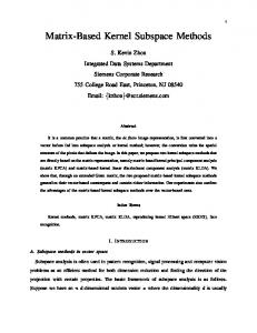
Thus the compressed matrix m = M2 requires less memory than the conventional storage of M as a 64-bit integer array. An illustration of the compression process and the allocation of the elements of matrix M in the matrix m is shown in Figure 1. Note that the matrix m has fewer columns that the matrix M, then it demands less memory to be represented. We also emphasize that the bits which represent the value 700 is divided in two parts and stored in different strips in the matrix m.

Figure 1. Representation of the compression process and allocation of elements of matrix M in the matrix m. The strip of value 700 is divided in two parts and stores in different strips in the matrix m.

Method 2: Variable Length Blocks (VLB)

In the SM method, there is still waste of space since for elements smaller than the supremum, a number of bits remain unused. In the VLB method, the absolute minimal number of bits are used to store each value. However, if we are going to divide the bitstrings into variable length chunks, we also need to reserve some extra bits to represent the size of each chunk, otherwise the elements cannot be recovered once they are stored. Lets use again the matrix described in Equation 2, where the largest element is number 1023. Now instead of assigning one chunk of the bitstring to each element of m, we will assign two chunks: the first will store the number of bits required to store the element and the second will store the actual element. 4/32 PeerJ PrePrints | http://dx.doi.org/10.7287/peerj.preprints.849v1 | CC-BY 4.0 Open Access | rec: 23 Feb 2015, publ: 23 Feb 2015

The first chunk will have a fixed size, in this case, 4 bits. These 4 bits are the required space to store the bit-length of sup M, in this case, 10. Lets go through VLB compression step-by-step. The largest element of M is 1023. Its bit-length is 10 which in turn is 4 bits long in base 2 (1010). Thus the fixed size chunk is 4 bits long for every element. 1. The first element M1,1 = 900 requires 10 bits to store, so we write 10 in the first chunk and 900 in the second. bitstring1 = 00000000000000000000000000000000000000000000000000 1110000100 {z } |

1010 |{z }

element=900 bit-length=10

|

{z

}

M1,1

PrePrints

2. Do the same for the next element, M1,2 = 1023. bitstring1 = . . . 00000000000000000000000000 1111111111 | {z }

1010 | {z}

1110000100 | {z }

1010 |{z }

element=1023 bit-length=10 element=900 bit-length=10

|

}|

{z

M1,2

{z

}

M1,1

3. Element M1,3 = 721 is also added taking the bitstring to the state. bitstring1 = 0000000000000000000000 1011010001 | {z } 1010 | {z } 1010 | {z} 1111111111 | {z } 1110000100 | {z } 1010 |{z } 721

10

1023

10

900

10

So far the VLB method is more wasteful than the SM, but when we add M1,4 = 256, we start to save some space. 4. Element M1,4 = 256 is added. 5. Elements M1,5 = 1 and M1,6 = 10 are added requiring a total of 13 bits instead of 20 with the SM method. With the addition of these elements we require a second bitstring. bitstring1 = 0100 1 0001 | {z } 1010 |{z } |{z} |{z } 100000000 | {z } 1001 |{z } 1011010001 | {z } 1010 | {z} 1111111111 | {z } 1110000100 | {z } 1010 |{z } 4

1

1

256

9

721

1023

10

10

900

10

bitstring2 = 000000000000000000000000000000000000000000000000000000000000 1010 | {z} 10

6. The remaining two elements are added M1,7 = 700 and M1,8 = 20 in the second bit strip. bitstring2 = 00000000000000000000000000000000000 10100 | {z } 0101 | {z} 1010111100 | {z } 1010 |{z } 1010 |{z } 20

5

700

10

10

We used a total of 87 bits to store matrix m with the VLB method instead of 80 bits using the SM method. However, as shall be seen later, the VLB method will be the most efficient for most matrices. With the VLB method the resulting matrix is smaller than the original matrix. Compression Efficiency Compression efficiency depends of the data being compressed. Below, a formula for calculating compression efficiency is derived for both methods. They will be based on the following ratio:

η=

bits alocated − bits used bits alocated

(4)

Where bits allocated above mean total bits required for standard storage of the matrix, without compression, while bits used mean total bits requires to store the matrix after compression. From now on the efficiencies are denoted by η1 for the SM method and by η2 for the VLB method. 5/32 PeerJ PrePrints | http://dx.doi.org/10.7287/peerj.preprints.849v1 | CC-BY 4.0 Open Access | rec: 23 Feb 2015, publ: 23 Feb 2015

SM Method

Let Mr×c be the matrix we wish to compress. In comparison with a conventional allocation (64-bit integers), we can apply Equation 4 to calculate the efficiency of the SM method: 64 × rc − b(maxM) × rc 64 × rc 64 − b(maxM) = 64

η1 =

(5)

As we see in 5, η1 does not depend on size of the matrix, only on the bit-length of max M. If b(max M) = 64, η1 is 0, i.e., no compression is possible. On the other extreme, if the matrix is composed exclusively of 0s and 1s, maximal compression is achievable, η1 = 0.9843.

PrePrints

VLB Method

For the VLB method, compression depends on the value of each element of the matrix. In this method bit-length variability affects the compression ratio, so the formula will have to include this information. Let the rc elements of the matrix Mr×c be divided into g groups, each with fi numbers of bit-length bi = b(mi ). Thus fi is the frequency of each bit-length present in M. Let k = b(b(max M)), i.e., the bit length of the bit-length of max M. The efficiency η2 is shown below.

η2 =

64 × rc − ∑gi=1 (bi + k) × fi 64 × rc

(6)

We can further simplify Equation 6 to get at shorter expression for the compression ratio. 64 × rc − ∑gi=1 (bi × fi + k × fi ) 64 × rc 64 × rc − ∑gi=1 bi × fi − ∑gi=1 k × fi = 64 × rc 64 × rc − ∑gi=1 bi × fi − k × ∑gi=1 fi = 64 × rc

η2 =

Knowing that g

∑ fi = rc,

i=1

we can simplify the equation above, obtaining (7). 64 × rc − ∑gi=1 bi × fi − k × rc 64 × rc g b × fi k ∑ i = 1 − i=1 − 64 × rc 64

η2 =

(7)

For this method, the highest value obtained for the data compression is 0.9687, when b = 1 and k = 1. g

However, the lower value is defined by a range of values, such that the value of k =

∑i=1 bi × fi rc

− 64.

OPERATIONS We will explore in more detail, basic arithmetic operations (addition, subtraction, division and multiplication) over the elements of bitstring compressed arrays. We will consider integer matrices compressed via both the SM and the VLB methods, but the proposed methods can be applied to integers and real numbers with sign. In these operations, the most important aspect is the bit-length of the result in relation to those of the operands. As the operations are all done in binary, when the result bit-length increases, the resulting matrix will require more space to store and the operation in itself gets more complex, as in place operations are not possible. In the following examples, we will explore these kinds of operations. 6/32 PeerJ PrePrints | http://dx.doi.org/10.7287/peerj.preprints.849v1 | CC-BY 4.0 Open Access | rec: 23 Feb 2015, publ: 23 Feb 2015

OPERATIONS WITH SCALARS Addition In base 2 the carry over behavior is the same as we observe when operating with decimals, only the base is different. Adding 1 + 1 results in 0 and a carry over of 1, this is similar to the decimal sum 5 + 5 where we also have a carry over of 1. Other single digit additions in base 2 are: 1 + 0 = 1, 0 + 1 = 1, and 0 + 0 = 0. Consider the following addition n1 + n2 where n1 = 7 and n2 = 10. This addition is illustrated in table 2 in both decimal and binary. Note that, when we add 1 + 1, a carry over is generated to be added to bit on the left. In total, we generate three bits in carry over. In Table 3, we show the addition of 7 + 7 which generates a 4 bits long number. In integer additions, the results may, in the very least, be as long (in bits) as the greatest operand (for example 1 + 2 = 3), but is frequently longer.

PrePrints

Table 2. Comparing binary and decimal sum (7 + 10). Decimal

Binary

bit-length

7 10 17

11100 111 1010 10001

3 4 5

Carry Over n1 n2 Total

Table 3. Comparing binary and decimal sum of 7+7.

Carry n1 n1 Total

Decimal

Binary

7 7 14

1110 111 111 1110

Bit-length 3 3 4

Subtraction Depending of the number involved in this operation, the result may be negative. This fact alone generates the need for an extra bit to represent the sign (+ or −). The usual way to achieve this is to use the two’s complement (Flores, 1963) representation which has the advantage of making the addition subtraction and multiplication operation the same as those for unsigned binary numbers. This algorithm is actually implemented in CPUs. To exemplify let’s subtract 7 from 10. To make use of the same algorithm of the sum , we represent the operation as 10 + (−7). First we need to convert the operands to two’s complement representation (C2): • The numbers will require an extra bit in C2. Thus 7 which is 3 bits long in binary, will require 4 bits in C2. As 7 will be added to 10, the operands must be represented by 5 bits (4 bits to represent 10 plus one for the signal). Therefore 7 becomes 00111 (in one’s complement). • Now the bits in 7 are flipped, going from 00111 to 11000. • to the flipped number we add 1: 11000 + 1 = 11001, which is the C2 representation of −7 Once completed the conversion, we add the numbers (see table 4). Both operands require 5 bits because of C2. Most importantly, the left most bit generated by the carry over, is discarded. That happens because to operate in C2, the operands must have the same bit-length so any overflow in the result must be discarded. This operation would be possible without the use of C2 representation as 10 is greater than 7, and no signed integer is involved (see table 5 for this). In conclusion, in the worst case subtraction will require the same number of bits of the greatest operand, regardless of the use of C2 representation. As an example, consider the subtraction 7 − 1 (table 6). 7/32 PeerJ PrePrints | http://dx.doi.org/10.7287/peerj.preprints.849v1 | CC-BY 4.0 Open Access | rec: 23 Feb 2015, publ: 23 Feb 2015

Table 4. Two’s complement addition(subtraction) in decimal and binary.

Carry over n2 +(−n1 ) Total

Decimal

C2 Binary

10 +(-7) 3

110000 01010 11001 100011

Bit-length 5 5 5

PrePrints

Table 5. Standard binary subtraction.

Carry over n2 −n1 Total

Decimal

Binary

10 -7 3

0111 1010 111 11

Bit-length 4 3 2

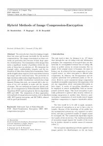
Multiplication If multiplication is thought of as a series of sums, we can apply much the same techniques. For example: 2 × 3 = 3 + 3 = 2 + 2 + 2. Table 7 describes a simple multiplication. In multiplication the behavior of the bit-length is different from the sum and subtraction. In the worst case, the product has a bit-length which is the sum of the bit-lengths of the factors. For example, in the product 7 × 7, the product is 6 bits long: 49 which in binary is 110001. If a signed integer is involved in the multiplication, we need to use C2 representation. To illustrate this case let’s calculate 10 × −7. in C2, this operation becomes 01010 × 11001. Table 8 contains the details. The basic difference is that the sign bits (in bold), positioned to the left, are not involved in the operation. Only in the end they are used to determine the sign of the product: 0 meaning positive and 1 negative. In the worst case the bit-length of the product is the sum of the bit-lengths of the factors plus 1 due to the sign. Division Division, in contrast to multiplication, requires successive subtractions until a remainder is reached which may or may not be zero. To illustrate the procedure in binary, table 9 describes the division of 50 by 10. Note the successive binary subtractions. The bit-length of the quotient is, in the worst case, equal to the bit-length of the dividend when this is longer than that of the divisor. With each subtraction, we add 1 to the quotient which is initially 0. The process ends when the remainder is 0 or less than the divisor. When the division involves a signed operand, we do the same as with the multiplication, the operations is executed on the unsigned operands and the sign is applied at the end. So far we have examined the 4 fundamental arithmetic operations. In summary the implication for memory allocation of the results are the following, in the worst case scenarios: • Addition: requires 1 extra bit above the bit-length of the greatest operand; • Subtraction: Requires the same number of bits as the greatest operand; • Multiplication: Requires the sum of the bit-lengths of the operands; • Division: Requires the same bit-length as the dividend; As can be seen in figure 2, the bit-lengths of results of the four operations with integer operands up to 8 bits in length. The conclusions listed above, are visually emphasized in the figures. When operating with signed integers, an extra bit is used for the sign. The operations on single numbers (scalars) as exposed above are a simplification of the actual operations taking place on the bitstrings as we compute with compressed matrices. Additional details will be provided below, when we discuss the operation with matrices. Note that we are restricting the example to operations which generate integer results. Handling of float operations and compression will be the subject of a subsequent paper. 8/32 PeerJ PrePrints | http://dx.doi.org/10.7287/peerj.preprints.849v1 | CC-BY 4.0 Open Access | rec: 23 Feb 2015, publ: 23 Feb 2015

Table 6. Binary subtraction Decimal

Binary

7 -1 6

000 111 1 110

Carry over n1 −n3 Total

Bit-length 3 1 3

PrePrints

Table 7. Binary Multiplication Decimal

Binary

n2 n1

10 ×7

Total

70

1010 111 1010 1010 11110 1010 1000110

Bit-length 4 3

7

OPERATION ON BITSTRINGS To illustrate operations with bitstrings, consider the matrices A an B, both 3 × 4: 

1 A = 12 3

3 5 14 6 7 10

 8 9 11

(8)

3 7 3 14 30 2

 9 15 1

(9)

and 

1 B=1 20

After bitstring compression by the SM method, they become 3 × 1. They are show in decimal and binary from in 10 and 11. The elements in A and B are 4 and 5 bits long, respectively (the “supreme minimum”). The ellipses (“. . .”) in the binary matrix correspond the extra zeros to the left. Since the strings are written into 64 bits integers, sometimes we end up with unused bits to the left.   . . . 0001} 0011 |{z } 0101 | {z} 1000 | {z}    |{z 1 3 8  5 4952 . . . 0001001101011000   . . . 1100 1110 0110 1001   AA = 52841 = . . . 1100111001101001 =  |{z } |{z } | {z} | {z}  12 14 9  6 14251 . . . 0011011110101011 . . . 0011 0111 1010 1011 |{z } |{z } | {z} | {z} 



3

7

10

(10)

11

and   . . . 00001 | {z } 00011 | {z } 00111 | {z } 01001 | {z }      1 3 7 59  36073 . . . 00001000110011101001   . . . 00001 00011 01110 01111   BB =  36303  = . . . 00001000110111001111 =  | {z } | {z } | {z } | {z }  1 3 14 15  . . . 10100111100001000001 686145 . . . 10100  11110 00010 00001 | {z } | {z } | {z } | {z } 20

30

2

(11)

1


Table 8. Multiplication involving a signed integer.

n2 × − 1n1

PrePrints

Total

Decimal

Binary

10 ×−7

01010 11001 1010 + 0000 01010 + 0000 001010 + 1010 11011010

-70

Bit-length 5 5

8

Table 9. Binary division as a series of subtractions.

n4 n2 Remainder n2 Remainder n2 Remainder n2 Remainder n2 Remainder

Decimal

Binary

Decimal quotient

Binary quotient

50 -10 40 -10 30 -10 20 -10 10 -10 0

110010 001010 101000 001010 011110 001010 010100 001010 001010 001010 000000

0 +1 1 +1 2 +1 3 +1 4 +1 5

000 +001 001 +001 010 +001 011 +001 100 +001 101

Consider now just the bitstring stored in the first line of each matrix (AA and BB). To recover the original elements we need to now the bit-length of the blocks of memory containing them, for the SM method they are all the same length. To obtain the values in an efficient way, we will use a binary mask. The mask will recover the first and third blocks at the same time to save time. The mask is stored as a bitstring the same length as those storing the matrix elements. The mask for the first and third elements of matrix AA is depicted in 12. To recover the second and fourth elements, we apply the mask shown on 13. For Matrix BB, see 14 and 15 for the respective masks.

Matrix AA’s mask for positions 1 and 3 = . . . 0000111100001111

(12)

Matrix AA’s mask for positions 2 and 4 = . . . 1111000011110000

(13)

Matrix BB’s mask for positions 1 and 3 = . . . 00000111110000011111

(14)

Matrix BB’s mask for positions 2 and 4 = . . . 11111000001111100000

(15)

Once defined the mask we can apply it to matrices A and B. We use the mask by applying the boolean function AND. Let tempA and tempB the recovered elements. The recovering process is illustrated below. Note that only the positions where the mask is 1 are retained. 10/32 PeerJ PrePrints | http://dx.doi.org/10.7287/peerj.preprints.849v1 | CC-BY 4.0 Open Access | rec: 23 Feb 2015, publ: 23 Feb 2015

PrePrints

Figure 2. Bit-length of the results for each of the four operations. The axes represent the values of the operands.

A[1, 1] = . . . 0001|0011|0101|1000 mask A = . . . 0000|1111|0000|1111 tempA = . . . 0000|0011|0000|1000

B[1, 1] = . . . 00001|00011|00111|01001 mask B = . . . 00000|11111|00000|11111 tempB = . . . 00000|00011|00000|01001 Addition Suppose we want to add both matrices and store it in a matrix S. for that the blocks of tempA and tempB must have the same length. As for the addition we need, in the worst case, an extra bit, the block length of the resulting bitstring will be 6. The string from each matrix, padded on the left towards this new length, are shown in equations 16 and 17. tempA = . . . 000000000011000000001000

(16)

tempB = . . . 000000000011000000001001

(17) 11/32


Now that the blocks are matched in length we can perform the operation S[1, 1] = tempA + tempB. The operation is repeated for the second and fourth regions. these operations can be done in parallel and the result, S[1, 1], is already in compressed form. tempA = . . . 000001|000011|000101|001000 tempB = . . . 000001|000011|000111|001001 S[1, 1] = . . . 000010|000110|001100|010001 We can see below the same operation performed for bitstrings S[2, 1] and S[3, 1]. tempA = . . . 001100|001110|000110|001001

PrePrints

tempB = . . . 000001|000011|001110|001111 S[2, 1] = . . . 001101|010001|010100|011000

tempA = . . . 000011|000111|001010|001011 tempB = . . . 010100|011110|000010|000001 S[3, 1] = . . . 010111|100101|001100|001100 Therefore, as the final result of the operation S = A + B, we have: 

   549649 . . . 000010000110001100010001 S =  274889  = . . . 000001000011000111001001 6181644 . . . 010111100101001100001100   . . . 000010 | {z } 001100 | {z } 010001 | {z } | {z } 000110   2 12 17 6   010001 010100 011000  . . . 001101 =  | {z } | {z } | {z } | {z }   13 17 20 24  . . . 010111 100101 001100 001100 | {z } | {z } | {z } | {z } 23

37

12

(18)

12

Subtraction To perform the subtraction, we need to use C2 notation. Suppose we need to calculate D = B − A. This operation can be done in the same way, by converting it to an addition: D = B + (−A), where −A will be converted to C2 (equation 19). Note the elements will be calculated with six digits. 

   4952 . . . 111111111101111011111000 −A = 52841 = . . . 110100110010111010110111 14251 . . . 111101111001110110110101   . . . 111111 | {z } 111101 | {z } 111000 | {z } 111011 | {z }   −1 −3 −8  −5  . . . 110100 110010 111010 110111 | {z } | {z } | {z } | {z } =   −12 −14 −9  −6  . . . 111101 111001 110110 110101 | {z } | {z } | {z } | {z } −3

−7

−10

(19)

−11

Now we apply the masks as before, but before we need to convert to C2 as well, in order to perform the addition. To exemplify, let’s examine closely the operations B[1, 1] + (−A[1, 1]), B[2, 1] + (−A[2, 1]) and B[3, 1] + (−A[3, 1]). We use tempB to store each line of the matrix B converted to C2. The numbers 1 marked in the bitstring, are overflows and must be removed. The result is shown below: 12/32 PeerJ PrePrints | http://dx.doi.org/10.7287/peerj.preprints.849v1 | CC-BY 4.0 Open Access | rec: 23 Feb 2015, publ: 23 Feb 2015

tempB = . . . 000001|000011|000111|001001 +(−A[1, 1]) = . . . 111111|111101|111011|111000 D[1, 1] = . . . 1000000|1000000|1000010|1000001

tempB = . . . 000001|000011|001110|001111 +(−A[2, 1]) = . . . 110100|110010|111010|110111

PrePrints

D[2, 1] = . . . 110101|110101|1001000|1000110

tempB = . . . 010100|011110|000010|000001 +(−A[3, 1]) = . . . 111101|111001|110110|110101 D[3, 1] = . . . 1010001|1110111|1111000|110110 After the removal of the overflows, matrix D becomes:    129 . . . 000000000000000010000001 D = 14111238 = . . . 110101110101001000000110 4685366 . . . 010001110111111000110110   000000 000010 000001 . . . 000000 | | | {z } {z } {z } {z } |   0 0 2 1   . . . 110101 110101 001000 000110   | {z } | {z } | {z } | {z } =  −11 −11 8 6   . . . 010001 110111 111000 110110 | {z } | {z } | {z } | {z } 

17

−8

23

(20)

−10

Multiplication Let’s now examine matrix multiplication. Consider the product P = A × Bt , where Bt is the transpose of B. Thus the product becomes:



1 P = A × B = 12 3

 1 8 3 9 × 7 11 9 

3 5 14 6 7 10

1 3 14 15

 20 30  2 1

(21)

Again, using AA and BB to denote the compressed versions of the matrices, and ×× to denote the multiplication of bitstring matrices, the compressed product becomes: 

 4952 P = AA × BB = 52841 × × 36073 14251

36303

  . . . 0001 |{z } 0011 |{z } 0101 |{z } 1000 | {z}  1 3 8  5   1110 0110 1001  . . . 1100 P = AA × BB =  |{z } |{z } |{z } | {z}  12 14 9  6 . . . 0011  0111 1010 1011 |{z } |{z } |{z } | {z} 3

7

10

686145

(22)

(23)

11


××

. . . 00001 | {z } 00011 | {z } 00111 | {z } 01001 | {z }

PrePrints

1

3

7

9

. . . 00001 | {z } 00011 | {z } 01110 | {z } 01111 | {z } 1

3

14

15

. . . 10100 | {z } 11110 | {z } 00010 | {z } 00001 | {z } 20

30

2

1

To calculate P[1, 1] which in uncompressed form is 1 × 1 + 3 × 3 + 5 × 7 + 8 × 9, we first must extract the numbers from the bitstrings and then proceed with the linear combination. The extraction will make use of masks as described before. Let tempA and tempB store the values of blocks 1 and 3 of AA[1,1] and BB[1,1]. Now we need to determine the size of the blocks (bit-length) containing each element of the resulting matrix. As demonstrated before, in the worst case, the product will have a bit-length which is the sum of the bit-lengths of the operands. For this example this length is 4 + 5 = 9, however, we also have three additions for each element,adding a total of 3 extra bits, thus we end up with a bit-length of 12 for each element of the product. Having determined the bit-length of the product, we can now do the actual calculations and store the results. The linear combination of elements which generates P[1, 1] is detailed below. We use temporary variables tempPi to store the products before adding them, where i is the product being calculated. tempA = . . . 0001|0011|0101|1000 tempB = . . . 00001|00011|00111|01001

tempA = . . . 0001|0011|0101|1000 tempB = . . . 00001|00011|00111|01001 tempP1 = . . . 000000001




tempP1 = . . . 0000000001 tempP2 = . . . 0000001001 sum = . . . 0000001010 (10 bits)

tempP3 = . . . 00000100011 sum = . . . 00000001010 sum = . . . 00000101101 (11 bits) 14/32 PeerJ PrePrints | http://dx.doi.org/10.7287/peerj.preprints.849v1 | CC-BY 4.0 Open Access | rec: 23 Feb 2015, publ: 23 Feb 2015

tempP4 = . . . 000001001000 sum = . . . 000000101101 sum = . . . 000001110101 (12 bits)

PrePrints

So, P[1, 1] is 000001010101, and the entire matrix P becomes:     1426882688 . . . 000001010101000011001000000010000000 P = 2970686121 = . . . 000010110001000100010001001010101001 3239350573 . . . 000011000001000101001001000100101101   . . . 000001010101 | | | {z } 000011001000 {z } 000010000000 {z }   117 200 128   000100010001 001010101001 . . . 000010110001 {z }| {z }| {z } = |    177 273 681  . . . 000011000001 000101001001 000100101101 | {z }| {z }| {z } 193

329

(24)

301

Again, we can see that P is already in compressed form, which confirms that the entire operation was conducted without decompressing the data. The division operation with matrices will be described in a subsequent paper after we describe how to represent and operate with floating-point numbers. In the examples given above, we only used the SM method, but the same procedure can be easily adapted to the VLB method. Thus we complete our demonstration of how to perform basic arithmetic operations with bitstring compressed scalars and matrices.

RESULTS In both methods, compression efficiency depends on the distribution of the bit-lengths b(mi, j ). Thus, in this section, a method to generate a variety of random bit-length distributions is proposed. For simplicity we will model the distribution of as a mixture X of two Beta distributions, B1 ∼ Beta(α1 , β1 ) and B2 ∼ Beta(α2 , β2 ), whose probability function is shown in Equation 25. Since the Beta distribution is defined only in the interval [0, 1] ⊂ R , we applied a simple transformation (b64 × xc + 1) to the mixture in order to map it to the interval of [1, 64] ⊂ Z. Random Matrix Generation

f (x) = w Beta(α1 , β1 ) + (1 − w) Beta(α2 , β2 )

(25)

The intention of using this mixture was to find a simple way to represent a large variety of bit length distributions. The first two central moments of this mixture are given in 26 and it will be used later to summarize our numerical results. E(X) = wE(B1 ) + (1 − w)E(B2 ) α1 α2 + (1 − w) =w α1 + β1 α2 + β2 Var(X) = wVar(B1 ) + (1 − w)Var(B2 ) + w(1 − w)(E(B1 )2 − E(B2 )2 )

(26)

In order to explore the compression efficiency of both methods, we generated samples from the mixture defined above, varying its parameters. From now on, when we mention Beta distribution we will mean the transformed version defined above. From now on, we will apply Equations 5 and 7, to determine the compression efficiency of SM and VLB methods for random matrices generated as describe above. 15/32 PeerJ PrePrints | http://dx.doi.org/10.7287/peerj.preprints.849v1 | CC-BY 4.0 Open Access | rec: 23 Feb 2015, publ: 23 Feb 2015

4000 3000

250

2000

Frequency

200 150

Frequency

1000

100

0

50 0

1

8

16

24

32

40

48

56

64

1

8

16

24

Bit number

32

40

48

56

64

48

56

64

Bit number

(b) α = 1, β = 32

800 400

600

Frequency

1000

3000 2000

Frequency

0

200

1000 0

PrePrints

1200

4000

1400

(a) α = 1, β1 = 1

1

8

16

24

32

40

Bit number

(c) α = 32, β = 1

48

56

64

1

8

16

24

32

40

Bit number

(d) α = 64, β = 64

Figure 3. Histograms constructed from samples with 10,000 elements, generated from a Beta distribution. Below each histogram is possible to verify the parameters used.With these two parameters it is possible to perform different combinations of numbers to fill the arrays to be compressed. With w = 0, a single Beta distribution is used. In Figure 3, we show some distributions of bit-lengths for some combinations of α1 and β1 . From the figure it can be seen that a large variety of unimodal distributions can be generated in the interval [1, 64]. As we are sampling from a large set distributions of bit-length, represented by the mixture of betas presented above, in order to make our results more general, we will base our analysis on the expected bit-length of a sample, since the efficiency of both methods depends on it. So, from Equations 5 and 7, the expected efficiencies become:

E(η1 ) = 1 −

k 64

(27)

E(η2 ) = 1 −

E(b) k − 64 64

(28)

where k, in (28), is set to 7 (the bit-length required to represent the largest possible bit-length: 64). In (27), k is the bit-length of the greatest element, or in the worst case, 64. We will use the difference D = E(η1 ) − E(η2 ) to compare the efficiency of the two methods. Thus a positive D will favor SM method while a negative D favors VLB method. The expected compression efficiency in the following numeric experiments, will be calculated from 3 matrices of dimension 10, 000, generated as described, and presented in tables and figures below. In Figure 4, we can see the distribution of efficiencies and their difference for a sample generated from a single Beta distribution of bit-lengths. Note that both methods can achieve efficiencies greater than 80% for matrices with very small numbers. Also note that the VLB method is more efficient in the majority of cases. Now let w = 0.5, i.e., matrices will have elements with bit-lengths coming from a mixture of beta distributions, B1 ∼ Beta(α1 , β1 ) and B2 ∼ Beta(α2 , β2 ). The expected value for this mixture is shown in Equation 29. 16/32 PeerJ PrePrints | http://dx.doi.org/10.7287/peerj.preprints.849v1 | CC-BY 4.0 Open Access | rec: 23 Feb 2015, publ: 23 Feb 2015

56

56

48

48

0.8 0.0 40

40 0.7

−0.1 0.6

−0.3

32

32 0.5

η1

η1 −η2

−0.2

0.4

24

24

0.3

−0.4 0.2 −0.5 16

10

0.1

10

20

16

20 30

α

30

α

60

40

50 8

40

50

50 8

30 20

60

β

10

40

50

30 20

60

60

40

(a) SM-VLB Difference (D = η1 − η2 )

β

10

(b) SM Efficiency (η1 ) 56

56

48

48

0.030 0.8 40

40 0.025

0.6 0.020

≥η2

32

0.015

η1

0.4

η2

32

24

24 0.010

0.2

PrePrints

0.005 16

10

0.0 20

16

10 20

30

α

0.000 30

60

40

50 40

50

30 20

60

10

β

(c) VLB Efficiency (η2 )

8

α

60

40

50 40

50

8

30 60

20 10

β

(d) SM≥VLB Efficiency (η1 ≥ η2 )

Figure 4. Comparing compression efficiency of methods 1 and 2. Color scale in represent average bit-length. In (a) we can see the difference D = η1 − η2 . It can be seen that for most combination of α and β , D < 0, meaning the second method is more efficient to compress a sample of numbers with bit-lengths coming from a Beta(α, β ) distribution. However, there is a small region in parameter space, which is shown in white on (d), where the SM method is more efficient. This region corresponds to the dots in red in (a), where the average bit-length is higher. In panels (b) and (c), we can see the efficiencies of SM and VLB methods, respectively.

E(B) = 0.5E(B1 ) + 0.5E(B2 )

(29)

For bit-lengths coming from a mixture (w > 0), let the expected efficiencies for the SM and VLB methods be as given by Equations 30 and 31. So now, instead of having the efficiency be a function of greatest bit-length in the sample (denoted as k in 5 and 7), it will be a function of max{E(B1 ), E(B2 )}.

E(η1 ) = 1 −

max{E(B1 ), E(B2 )} 64

E(η2 ) = 1 − 0.5

E(B1 ) E(B2 ) max{E(B1 ), E(B2 )} − 0.5 − 64 64 64

(30)

(31)

As before, we generate 3 matrices of dimension 10, 000 for each parameterization, calculate the average efficiencies (Equations 30 and 31) and their difference D. Before moving on to efficiency results and analyses, let’s first inspect samples from the mixture of transformed Beta distributions. Figures 5 and 6, show a few parameterizations and their resulting sample distributions. It is important to note that from the mixture, we can now generate bimodal distributions as well as the unimodal types tested before. Since we are making statements about efficiency as a function of the expected bit-length, it is important to verify if these statements hold for bimodal distributions as well. After sampling uniformly ([1, 5, 9, . . . , 64], n = 65, 536) the bit-length space and comparing efficiencies, we summarized the results on Table 10. In it we see how many parameterizations (from our sample) favor each method. We can also look at the distribution of efficiencies on our samples for each method (Figure 7), which clearly demonstrate the greater expected efficiency of method VLB (Figure 7(b)). As we have shown, the VLB method is more effective compressing most integer datasets up to 64 bits in size. This is due to its ability to exploit the variance in the data set and reduce the waste of bits in the 17/32 PeerJ PrePrints | http://dx.doi.org/10.7287/peerj.preprints.849v1 | CC-BY 4.0 Open Access | rec: 23 Feb 2015, publ: 23 Feb 2015

40000 30000

1500

0

10000

20000

Frequency

1000 Frequency 500 0

1

8

16

24

32

40

48

56

64

1

8

16

24

Bit number

48

56

64

12000 Frequency

0

0

2000

2000

4000

6000

8000

10000

8000 6000 4000

Frequency

40

(b) α1 = 1, β1 = 32, α2 = 32, β2 = 1

10000

(a) α1 = 1, β1 = 1, α2 = 1, β2 = 1

PrePrints

32 Bit number

1

8

16

24

32

40

48

56

64

1

8

16

Bit number

24

32

40

48

56

64

Bit number

(c) α1 = 32, β1 = 32, α2 = 32, β2 = 32

(d) α1 = 64, β1 = 32, α2 = 32, β2 = 64

Figure 5. Histograms constructed from samples with 10,000 elements, generated from the mixture of two Beta distributions with w = 0.5. Below each histogram are the parameters of the mixture. Table 10. Efficiency comparison of SM and VLB methods for parameters covering uniformly the support of B. Column n shows the number of parameter combinations with which each method has superior compression. Methods

n

Percentage

SM VLB

592 64944

0.9034% 99.0966%

Total

65536

100%

representation of some numbers. In specific cases, where the variance in the data null or too small, method I will be more efficient. As a matter of fact, for matrices where all elements have the same bit-length, SM method will always be better, regardless of bit-length (Figures 8(a) and 8(b)). There are only one exception: for bit-length 64, where neither method is able to compress the data.

DISCUSSION Calculating Efficiencies To determine the best compression method to apply, it’s necessary to inspect the distribution of bit-lengths of matrix elements. When matrix elements are small or have nearly-constant bit-length, the SM method is better, otherwise, the VLB method should be chosen. As an example, let Mr×c be a integer matrix, such that the half of its elements have bit-length 1 and the other half 64. Recalling Equation 7, now we have two groups of elements (by bit-length), b1 = 1, b2 = 64 and fi = rc2 for i = 1 and 2. As the greatest bit-length is 64, then k = 7. Compression efficiency η2 can be calculated using Equation 7. After plugging in our numbers, we obtain a compression of 38.29%.

η2 = 1 −

7 ∑2i=1 bi × fi − 64 × rc 64 18/32


6000

25000

Frequency

3000

4000

5000

20000 15000

Frequency

2000

10000

1000

5000

0

0

1

8

16

24

32

40

48

56

64

1

8

16

24

Bit number

32

40

48

56

64

Bit number

(b) α1 = 16, β1 = 46, α2 = 49, β2 = 64

15000

Frequency

10000

3000

Frequency

5000

2000

0

1000 0

PrePrints

4000

20000

5000

25000

6000

(a) α1 = 64, β1 = 48, α2 = 1, β2 = 48

1

8

16

24

32

40

48

56

Bit number

(c) α1 = 16, β1 = 16, α2 = 16, β2 = 49

64

1

8

16

24

32

40

48

56

64

Bit number

(d) α1 = 1, β1 = 16, α2 = 1, β2 = 49

Figure 6. Histograms constructed from samples with 10,000 elements, generated from the mixture of two Beta distributions with w = 0.5. Below each histogram are the parameters of the mixture.

η2 = 1 −

1 × rc2 + 64 × rc2 7 − 64 × rc 64

η2 = 1 −

7 32.5 × rc − 64 × rc 64

η2 ≈ 1 − 0.5078 − 0.1093

η2 ≈ 38.29% The efficiency of the VLB method is influenced by the relative size of the bit-length groups. In this first example, we considered only two groups, each comprised of half the matrix elements. Let’s now vary the relative frequency of the groups, rcfi , while sticking to two groups. Here, we assume that rcfi is a good approximation to the probability of a given bit-length in a matrix, which we will denote by pi . With this definition, we can rewrite the Equation 7, which becomes 32. In Equation 32, the rcfi is replaced by pi , representing the probability of elements from group i in matrix M. g

η2 = 1 −

k ∑i=1 bi × pi − 64 64

(32)

with

pi =

fi rc

(33) 19/32


Frequency

0

2000

4000

6000

15000 10000

Frequency

5000 0

0.0

0.2

0.4

0.6

0.8

1.0

0.0

0.2

0.4

Efficiency

0.6

0.8

1.0

Efficiency

(a) Efficiency histogram of the SM method

(b) Efficiency histogram of the VLB method

Figure 7. Efficiency histograms of the SM and VLB methods. Note that the VLB method has a greater average efficiency than SM method. 0.1 SM Method VLB Method 0.08

0.6

0.06 Efficient

0.8

Efficient

PrePrints

1

0.4

0.04

0.2

0.02

0

0

10

20

30

40

50

60

70

bit

(a) Efficiencies of the SM and VLB methods, for constant bit-length matrices.

0

8

16

24

32 Bit

40

48

56

64

(b) η1 − η2 for matrices of constant bit-length.

Figure 8. Compression efficiency of the SM and VLB methods for matrices of constant bit-length. With the Equation 32 can analyze the influence of bit-length probability in compression efficiency. In this example, p1 and p2 represent the probability of elements of bit-lengths 1 and 64, respectively. Thus, efficiency is defined in Equation 34.

η2 = 1 −

1 × p1 + 64 × p2 7 − 64 64

(34)

Now, we can determine which probabilities give us the best and worst compression levels. When η2 = 1, then the efficiency is maximal and if η2 = 0, a efficiency is minimal. To calculate the values of p1 and p2 for both extreme values of η2 , we must solve the linear systems shown in Equations 35 and 36. The first equation on both systems come from the law of total probability. The second comes from 34 after setting η2 to 1 and 0, respectively. η2 = 1 :

p1 + p2 = 1 p1 + 64p2 = 7

(35)

Solving the system above, we find that when p1 = 0.9047 and p2 = 0.0953, efficiency is maximal, and in this particular case is equal to 87.5%. η2 = 0 :

p1 + p2 = 1 p1 + 64p2 = 57

(36)

Thus, when p1 = 0.1111 and p2 = 0.8889 the efficiency is minimal for the VLB method. For other combinations see Table 11. Looking at this table, one can see two negative efficiencies, when (p1 ,p2 ) assume the values (0,1) and (0.1,0.9). This correspond th cases, when the method increases, the memory requirements instead of decreasing it. 20/32 PeerJ PrePrints | http://dx.doi.org/10.7287/peerj.preprints.849v1 | CC-BY 4.0 Open Access | rec: 23 Feb 2015, publ: 23 Feb 2015

PrePrints

Table 11. Combinations p1 and p2 to calculate the efficiency. p1

p2

η2

0.0 0.1 0.2 0.3 0.4 0.5 0.6 0.7 0.8 0.9 1.0

1.0 0.9 0.8 0.7 0.6 0.5 0.4 0.3 0.2 0.1 0.0

-0.109 -0.010 0.087 0.185 0.284 0.382 0.481 0.579 0.678 0.776 0.875

So far, we have examined only two groups (hence two probabilities) of bit-length for the sake of simplicity. Before, we generalize to probability distributions let’s take a quick look at the efficiencies for more groups, with uniform probability: • 3 groups with bit-lengths 1, 32 and 64 bits, efficiency η2 = 0.3854, • 5 groups with bit-lengths 1, 16, 32, 48 and 64 bits, efficiency η2 = 0.3875, • 8 groups with bit-lengths 1, 8, 16, 24, 32, 40, 48, 56 and 64 bits, efficiency η2 = 0.3888 When the distribution of the group probabilities is uniform, i.e., the groups have approximately the same size, efficiency is basically the same, regardless of the number of groups. Now, we can leverage the notion of bit-length probabilities, and study efficiency when bit-lengths follow some commonly used discrete probability distributions: Discrete Uniform, Binomial and Poisson. For all the experiments, we assume k = 7, that is, the maximum possible bit-length is 64 bits. Thus, efficiency obtained will not be the best possible, since for that we would need assume small values of k (Equation 32). Discrete Uniform Let the bit-lengths of the matrices be distribute according to the Uniform distribution U(a = 1, b = 64), 1 which means bit-lengths may take values in the set {1, 2, 3,. . . , 64} with equal probability, i.e., 64 . Let the random variable B ∼ U(a = 1, b = 64) represent the bit-length of the elements of matrix M. Then E(bi ) = ∑i bi × p(bi ) = a+b 2 . Applying this result to the expected compression efficiency of VLB method (Equation 32), we have

Theoretical Efficiency:

E(η2 ) = 1 −

E(B) k − 64 64

(37)

assuming all bit-lengths are possible, i.e., a = 1 and b = 64, and hence k = 7, we can calculate η2 :

E(η2 ) = 1 −

1+64 2

64

−

7 ≈ 38.28% 64

(38)

This result agrees with the numerical estimates presented in Table 12. Numerical Estimates: To calculate the VLB efficiency, we generated a matrices with 100 (M10×10 ), 10,000 (M100×100 ) and 1,000,000 (M1,000×1,000 ) elements with 1, 8, 16, 32 and 64 number of bits. The average efficiency (Table 11) is calculated from a 1,000 replicates of each matrix size. As expected the compression efficiency gets better with lower expected bit-length. 21/32 PeerJ PrePrints | http://dx.doi.org/10.7287/peerj.preprints.849v1 | CC-BY 4.0 Open Access | rec: 23 Feb 2015, publ: 23 Feb 2015

Table 12. Compression efficiency of VLB method of samples with bit-lengths coming from a Discrete Uniform distribution U(a = 1, b = 64). Average efficiency (η2 ± SD) were calculated over a 1,000 replicates.

PrePrints

Efficiency η2 Expected bit-length

100

Matrix Size 10,000

1,000,000

1 8 16 32 64

0.8750±0.0000 0.8202±0.0031 0.7580±0.0066 0.6330±0.0142 0.3826±0.0288

0.8750±0.0000 0.8203±0.0003 0.7578±0.0007 0.6329±0.0014 0.3828±0.0028

0.8750±0.0000 0.8203±0.0000 0.7578±0.0001 0.6328±0.0001 0.3828±0.0003

Binomial Distribution For the binomial distribution, we will use Bin(n, p), with the number of trials n representing the greatest possible bit-length in the matrix, and np giving us the expected bit-length. Let bit-length (B) be a random variable with Binomial distribution, B ∼ Bin(n = 64, p = 0.5), E(bi ) = ∑i bi × p(bi ) = n × p and the efficiency becomes (with k = 7): Theoretical Efficiency:

k 64 × p − 64 64 64 × 0.5 7 = 1− − ≈ 39.05% 64 64

E(η2 ) = 1 −

(39)

Which again agrees with estimates in Table 13. Table 13. Compression efficiency with bit-lengths distributed according to a binomial distribution Bin(n, 0.5). Parameter n ∈ {1, 8, 16, 32, 64} represents the maximum bit-length. Since p = 0.5 the expected bit-length is n/2 (first column) Efficiency η2 Expected bit-length

100

Matrix Size 1,000

1,000,000

1 8 16 32 64

0.8828±0.0004 0.8283±0.0022 0.7656±0.0032 0.6406±0.0045 0.3910±0.0065

0.8828±0.0004 0.8281±0.0002 0.7656±0.0003 0.6406±0.0004 0.3906±0.0006

0.8828±0.0000 0.8281±0.0000 0.7656±0.0000 0.6406±0.0000 0.3906±0.0001

For these experiments, the parameter n represents the maximum bit-length of matrix elements and takes values in {1, 8, 16, 32, 64}. In this case, we evaluate the efficiency as a function of the parameter n, and matrix size. Even though efficiency does not depend on matrix size, we tried different sizes to test the stability of the compression algorithm. Results are shown in Table 13. As expected, smaller bit-lengths lead to higher compression efficiencies. Numerical Estimates:

Poisson Distribution With bit-length derived from a Poisson(λ ), the parameter λ corresponds to the expected bit-length. For the purpose of this analysis this Poisson distribution is truncated at 64. Theoretical Efficiency:

Let bit-length B ∼ Poisson(λ = 32). In this case, E(bi ) = λ , with k = 7, the

efficiency becomes: 22/32 PeerJ PrePrints | http://dx.doi.org/10.7287/peerj.preprints.849v1 | CC-BY 4.0 Open Access | rec: 23 Feb 2015, publ: 23 Feb 2015

λ k − 64 64 32 7 = 1− − ≈ 39.06% 64 64

E(η2 ) = 1 −

(40) (41)

This result is in accordance to Table 14. Table 14. Compression efficiency with bit-lengths distributed according to a Poisson distribution (λ ), where λ represents the expected bit-length.

PrePrints

Efficiency η2 Expected bit-length

100

Matrix Size 1,000

1,000,000

1 8 16 32

0.8751±0.0015 0.7654±0.0046 0.6405±0.0064 0.3908±0.0087

0.8750±0.0004 0.7656±0.0005 0.6406±0.0006 0.3906±0.0009

0.8750±0.0000 0.7656±0.0000 0.6406±0.0001 0.3906±0.0001

The results for this simulation can be seen in table 14. Note that increasing the number of bits to represent numbers leads to a loss of efficiency in the compression process. In this case, we did not simulate for λ = 64 since a large portion of the samples would fall above the maximum bit-length. These results show that a good compression is guaranteed when bit-lengths are distributed according to the tested distributions regardless of sample size. Numerical Estimates:

IMPLEMENTATION This paper proposes bitstring-based compression methods. The SM method was implemented as a FORTRAN library (Supplementary Material) which is available under an open-source license. The implementation extends the standard Matrix type of FORTRAN, overloading operators such as assignment, addition, subtraction, multiplication, transpose, and maximum of a matrix. Although only few significant matrix operations have been overloaded in this example implementation, any other operation can be performed, since the methods for inserting and collecting an element in a matrix of bitstring were also implemented. With these two methods, as long as they are properly adapted into algorithms, it is possible to implement any other desired operation. The SM method was also extended to allow for the allocation of real and signed integer matrices, besides positive integer ones. Some adjustments were made so that the other types of numbers could be represented. The SM method uses a fixed number of bits to store the values in such a way that the size or number of bits used is important to represent the highest value in the bitstring matrix. The adaptation consists in determining the largest value to be stored considering the absolute value of the number. That done, when the number is negative, it is necessary to rewrite it since, due to the sign, this will be written in the form of two’s complement. The purpose of this conversion is to optimize library processing. Take the following as an example: the number 5, when represented in a 32-bit integer, is defined as:

5 = 00000000000000000000000000000101 However, if the number is negative, this is represented in the form of two’s complement. Therefore, the number -5 is represented as: −5 = 11111111111111111111111111111011 23/32 PeerJ PrePrints | http://dx.doi.org/10.7287/peerj.preprints.849v1 | CC-BY 4.0 Open Access | rec: 23 Feb 2015, publ: 23 Feb 2015

PrePrints

Note that the bit positioned more to the left should be used to inform that the number is -5. For the purpose of optimization of the library, it was chosen to conversion of positive numbers to negative numbers and use of 1 bit to represent the sign. In turn, in order to represent real numbers, a conversion procedure of real numbers to integer numbers was used. The real number is multiplied by a power of ten and is then immediately truncated. The real numbers in a binary system of 64 bits are represented using a bit to represent the sign of the number, 11 bits to the exponent, and 52 bits to the mantissa. Note that 1 bit is still used implicitly, according to the IEEE-754 standard. In summary, the mantissa is represented in the base 2−1 , 2−2 , 2−3 , . . ., 2−52 . Depending on the value to be represented, loss of information can take place, which is related to the accuracy of the type used. In this case, considering a real number with double precision, the demand of 64 bits to represent each one occurs, and in some cases, the number to be represented is an approximation. As an example, consider that the number to be stored is 1.109. Following the traditional system, the number 1.109 is represented by 0011111111110001101111100111011011001000101101000011100101011000 We consider that the power used is 103 , that is, the number which needs to be stored would be 1109. In binary, that number is represented by 10001010101. Note that the number of bits required is smaller, but depending on numerical accuracy, the compression methods suggested are ineffective. When the power of 10 is used, it must be applied across the matrix. This conversion allows the proposed methods to be applied to a set of real numbers. It should be taken into account that the greater the power of 10 used, which is associated with the conversion of the real number, the larger the set of bits will be required to represent the converted number. This affects the efficiency of data compression. The use of the library to represent real numbers is conditioned to a study of the necessary level of precision to solve the problem.

DEMONSTRATION LIBRARY AND SAMPLE APPLICATIONS We implemented a simple library (Supplementary Material) along with some sample applications involving elementary matrix operations in order to benchmark our compression methods against standard matrix libraries. The application are: the attribution of a constant to all the elements of a matrix; the addition, subtraction and multiplication of all elements by a constant; the addition, subtraction and multiplication of matrices. In addition to that, the calculation of the transposed matrix and the maximum of the matrix were also considered. One of the characteristics of bitstring matrices is that the operations per column, in the case of implementation in FORTRAN, can be parallelized. This reduces the execution time, compared to traditional methods. Therefore, in order to achieve this optimization, threads were used for the implemented operations. We performed the comparisons under various square matrix dimensions nxn, with n = 10, 100, 1, 000, 10, 000, 20, 000 to 100, 000, so that a matrix created with a n = 1, 000 has 106 elements, while the one with n = 100, 000 has 1010 elements. With the increase of the size of the matrices, a larger amount of memory must be used to allocate the numbers. In Figures 9 and 10 the results from the processing time (in milliseconds) for the operations that involved only integer (Z) and positive integer numbers (Z + ) are represented. The traditional method (Normal) and the Bitstring method (Bitstring Z, integer numbers and Bitstring Zp, positive integer numbers) were used. The operations were attribution (A = 5, A is a matrix with dimension n by n); sum of the elements of a matrix with a constant (A = A + 5); sum of matrices (A = A + A); and subtraction of the elements of a matrix with a constant (A = A − 8). These operations are represented in Figure 9. Figure 10, in turn, shows the results for the multiplication operations of matrices (A = A × A); for the multiplication of the the elements of a matrix by a constant (A = A × 2); and for the calculation of transpose and maximum of a matrix. The results show that the bitstring method is faster than the traditional ones only for the attribution. This occurs because the element of the matrix is used more than once to store the numbers, differently from the traditional method. Due to the number of manipulations the bitstring method does, the other operations demand more time to be processed, but this can be optimized. When applied to positive integers, the bitstring model works faster than when applied to integers because it does not need to do operations related to the signals. 24/32 PeerJ PrePrints | http://dx.doi.org/10.7287/peerj.preprints.849v1 | CC-BY 4.0 Open Access | rec: 23 Feb 2015, publ: 23 Feb 2015

2.5 2 1.5 1 0.5

Processing Time

Normal Bitstring Z Bitstring Zp

0

Processing Time

0.2 0.4 0.6 0.8 0


10

10000

20000

10

10000

Dimension n

20000

Dimension n

(b) A = A + 5

2 1.5 1

Processing Time


0

0.5

3 2 1

Processing Time


0

PrePrints

2.5

(a) A = 5

10

10000 Dimension n

(c) A = A + A

20000

10

10000

20000

Dimension n

(d) A = A − 8

Figure 9. Processing time of the following operations: attribution (A = 5, A is the matrix with an n by n dimension); element sum of a matrix with a constant (A = A + 5);sum of matrices (A = A + A); and subtraction of the elements of a matrix by a constant (A = A − 8) involving integer numbers (Z) and positive integer numbers (Z + ). The bitstring method presented the best overall performance only for the attribution operations, because the storage of different numbers occurs in one element of a matrix, which reduces the accessing time. For the other operations, the bitstring method is slower due to the number of operations which are necessary to be executed in order to access the elements. This can still be optimized in the implemented library.

The results for the real numbers are represented in Figures 11 and 12. By repeating the operations tested in the integer numbers, it was possible to see that the bitstring method cannot overcome the traditional method. This happens because its application to the real numbers, as alternative to maintain the compression, asks for a conversion of real to integer numbers in order for them to be stored and when accessed, another conversion is made. This is a problem from the implementation process, but it can be optimized. Another library application was the implementation of the algorithm in order to deal with the problem of arrays of collaborative filtering (Lemire and Maclachlan, 2007). These arrays have large dimensions due to the number of users and products. Each element of this matrix stores the rating of a user with respect to a specific product. With this information, it is possible to specify a product for a determined customer. The manipulation of these matrices, depending on the amount of memory to be allocated, are one of the possible applications of the methods proposed in this work, since it promotes the compression and data allocation in the main memory. The allocation of the matrix within the main memory makes the access time to the elements much smaller than when the matrix is stored in secondary memory. This latter type of storage is used in some already mentioned techniques. As an example, let us examine the manipulation of a CF matrix, evaluating the access time to the elements and especially the size of the memory required to run such operation. The algorithms applied to this matrix were the average per-use and the bias from mean (Lemire and Maclachlan, 2007), this last one of the simplest algorithms for predicting the rate of users. An example of the application of the methodology presented is shown in Figure 13. In this figure, the matrix with normal and bitstring formats are displayed. In both matrices, the information is represented and can be accessed. Therefore, it becomes possible to apply the selected algorithms. In order to test a possible model application, we considered a matrix with the following dimensions: 25/32 PeerJ PrePrints | http://dx.doi.org/10.7287/peerj.preprints.849v1 | CC-BY 4.0 Open Access | rec: 23 Feb 2015, publ: 23 Feb 2015

3 2


0

1

Processing Time

40000 25000

Processing Time

0

10000


10

10000

20000

10

10000

Dimension n

20 10

10000 Dimension n

(c) transpose(A)

20000

50


30

40

60


0 10

Processing Time

70

80 100

(b) A = A × 2

0

Processing Time

(a) A = A × A

PrePrints

20000

Dimension n

10

10000

20000

Dimension n

(d) maximum(A)

Figure 10. Processing time of matrix multiplication (A = A × A, A is the matrix with a n by n dimension), element multiplication of matrix by constant (A = A × 2), the calculation of transpose and maximum of a matrix involve integer numbers (Z) and positive integer numbers (Z + ). In this cases, the traditional method was faster than the bitstring model.

95,000 users (lines) by 3,000 movies (columns), with the ratings for Netflix’s movies 1 . In order to evaluate a larger dataset, we modified the NetFlix data so we could increase the dimension of the matrix to be analyzed. The 95,000 users correspond to the lines of the matrix. In order to gradually increase the number of lines, we performed consecutive re-samplings and added them to the original matrix . As a results, we obtained a matrix with 600,000 lines and 3,000 columns. The operations used with the matrix were the Per User Average (PUA) and the rating estimation of a movie i using the Bias From Mean (BFM) (Lemire and Maclachlan, 2007). The analyses were made, considering the created matrix with different dimensions, with n from 40,000 to 600,000 by 20,000. It is important to emphasize that the number of columns is constant and equal to 3,000. The implementations of this problem were made in FORTRAN and both the developed library based in the method SM and in the traditional form were used. Codes were inserted in the library in order to optimize the multi-core processing using threads. No additional configuration was necessary to use the multi-core processing. since the library detects the characteristics of the processor uses them in the simulations. In turn, for the traditional implementation, we used the optimization process and parallelization, which are made available by the processor,as the vectorization and multi-core parallelization. The results are represented in Figures 14, 15 and 16 for the PUA Method and in Figures 17, 18 and 19 for the BFM Methods. A computer with 8 GB of RAM Memory, 16 GB of swap, processor core i7 model 870 and operational system Linux Debian 7.0 was used to perform this simulation. In Figure 14, it is possible to verify the approximate moment when the the storage in disk (swap) begins to be used. This is indicated by the vertical green line. At this moment, the bitstring method becomes faster than the traditional method because it does not require disk storage due to compressed memory representation. Note that, in the Figure 15, the traditional method is faster than the bitstring one before the beginning of the disk access. However, after it becomes necessary use the disk so that the matrix can be accessed and stored, the traditional method becomes slower (Figure 16). These results indicate that the bitstring method can promote the optimization of the memory use because the access to the main memories (RAM and cache) are faster than the access to secondary memories (disk). In Figures 17, 18 and 19 the results of the processing time for the BFM method are represented. Once again, a vertical green line indicates the 1 http://graphlab.org/downloads/datasets/


4 2

3

Normal Bitstring

0

1

Processing Time

0.6 0.2

0.4

Bitstring

0

Processing Time

Normal

10

10000

20000

10

10000

Dimension n

1.2

2.7

Bitstring

10

10000 Dimension n

(c) A = A + A

20000

2.1 3 3.9

Processing Time

4.2

Normal

Normal Bitstring

0 0.9

5.7

5.1

(b) A = A + 5.0000

0

Processing Time

(a) A = 5.0000

PrePrints

20000

Dimension n

10

10000

20000

Dimension n

(d) A = A − 8.0000

Figure 11. Processing time of the following operations: attribution (A = 5.0000, A is the matrix with an n by n dimension); element sum of a matrix with a constant (A = A + 5.000);sum of matrices (A = A + A); and subtraction of the elements of a matrix by a constant (A = A − 8.0000) involving real numbers (R) and positive integer numbers (R+ ). The bitstring method presented the best overall performance only for the attribution operations, because the storage of different numbers occurs in one element of a matrix, which reduces the accessing time. For the other operations, the bitstring method is slower due to the number of operations which are necessary to be executed in order to access the elements. This can still be optimized in the implemented library.

approximate moment when the disk access begins. There is a difference in relation to the PUA method since the BFM method uses the PUA values to perform its calculation. Therefore, the BFM method demands more memory to be processed, which reduces the matrix dimensions involved in the process, represented in the main memory. As indicated in Figure 16, for the PUA method, and Figure 19, for the BFM method, it is possible to verify that before the access to the disk, the traditional method is faster than the bitstring one, but once the access is initiated, the bitstring method becomes faster. In spite of the simplicity of the application, it is relevant since it allows for large-sized matrices to be allocated in memory and manipulated. We only implemented the SM method, as means to demonstrate the actual performance of the method. The VLB can also be implemented easily, however a bit more effort is required to do it efficiently. The example implementation was done in FORTRAN but it can just as easily be implemented in C or another efficient compiled language.

CONCLUSION In this paper, we have focused in the compression of matrix data, since this is one of the most important application the authors foresee. However, the compression methodology presented can be applied to any numerical data structure, with gains to performance and memory footprint (Paixão, 2012). Further discussions about doing computation with such compressed data-structures will be the subject of future work in which we will address details about the implementation of the compression algorithm, and benchmarks on classical linear algebra tasks such as those in Linpack(Dongarra, 1979). For the compression calculations presented in this paper we limited bit-length of integers to 64 bits. However the compression would work in the same way as discussed for computer architectures with larger word sizes. Representation of floating point numbers is also possible within the proposed compression framework, 27/32 PeerJ PrePrints | http://dx.doi.org/10.7287/peerj.preprints.849v1 | CC-BY 4.0 Open Access | rec: 23 Feb 2015, publ: 23 Feb 2015

5 4 3 2

Processing Time

Normal Bitstring

0

1

50000 20000

Bitstring

0

Processing Time

Normal

10

10000

20000

10

10000

Dimension n

(b) A = A × 2

(c) transpose(A)

20000

50

Bitstring

30

Processing Time 10000 Dimension n

Normal

0 10

Processing Time

20 40 60 80

Normal Bitstring

0

PrePrints

110

(a) A = A × A

10

20000

Dimension n

10

10000

20000

Dimension n

(d) maximum(A)

Figure 12. Processing time of matrix multiplication (A = A × A, A is the matrix with a n by n dimension), element multiplication of matrix by constant (A = A × 2.0000), the calculation of transpose and maximum of a matrix involve integer numbers (R) and positive integer numbers (R+ ). In this cases, the traditional method was faster than the bitstring model. but at the expense of precision in their representation. Although this may sound like a limitation, when we take into consideration that most experimental data have fewer “significant” digits than the maximal precision available in modern computers, fairly good compression may still be achievable for floats. Even though our demonstration library, without any optimization, performs worse than standard linear algebra libraries, it shows the ability to work with much larger matrices without incurring in memory swaps to disk. Given a properly optimized implementation, the methods presented in this paper may yield an interesting alternative for computations with very large matrices.

ACKNOWLEDGMENTS We would like to thank Claudia Torres Codeço, Moacyr Silva, Paulo Cezar Carvalho, Antonio Tavares da Costa Jr. and Carolina Bohórquez Grondona for fruitful discussions and key ideas which helped improve the manuscript.

REFERENCES Alted, F. (2010). Why modern cpus are starving and what can be done about it. Computing in Science & Engineering, 12(2):68–71. Bodden, E., Clasen, M., and Kneis, J. (2007). Arithmetic coding revealed. In Sable Technical Report 2007-5, Sable Research Group, School of Computer Science. (McGill University, Montréal. Dodson, D. S., Grimes, R. G., and Lewis, J. G. (1991). Sparse extensions to the fortran basic linear algebra subprograms. ACM Transactions on Mathematical Software (TOMS), 17(2):253–263. Dongarra, J. J. (1979). LINPACK users’ guide. Number 8. Siam. Flores, I. (1963). The logic of computer arithmetic, volume 1063. Prentice-Hall. Gaber, M. M., Zaslavsky, A., and Krishnaswamy, S. (2005). Mining data streams: a review. ACM Sigmod Record, 34(2):18–26. Kane, M. J. and Emerson, J. W. (2012). bigmemory: Manage massive matrices with shared memory and memory-mapped files. R package version 4.3.0. Lemire, D. and Maclachlan, A. (2007). Slope one predictors for online rating-based collaborative filtering. CoRR, abs/cs/0702144. 28/32 PeerJ PrePrints | http://dx.doi.org/10.7287/peerj.preprints.849v1 | CC-BY 4.0 Open Access | rec: 23 Feb 2015, publ: 23 Feb 2015

PrePrints

Figure 13. Illustration of the process of the bitstring model application to matrices of collaborative filtering of the algorithms per use average (PUA) and of the bias from mean (BFM) in a matrix represented in the traditional and bitstring formats. Lynch, C. (2008). Big data: How do your data grow? Nature, 455(7209):28–29. Paixão, C. A. (2012). Bitstring model for study of the propagation Dengue fever. Phd thesis, Federal University of Lavras. Salomon, D. (2007). Data Compression: The Complete Reference. Number v. 10 in Data compression: the complete reference. Springer-Verlag New York Incorporated, London. Salomon, D., Motta, G., and Bryant, D. (2009). Handbook of Data Compression. Springer, London. Van Der Walt, S., Colbert, S. C., and Varoquaux, G. (2011). The numpy array: a structure for efficient numerical computation. Computing in Science & Engineering, 13(2):22–30. Yemliha, T., Chen, G., Ozturk, O., Kandemir, M., and Degalahal, V. S. (2007). Compiler-directed code restructuring for operating with compressed arrays. In Proceedings of the 20th International Conference on VLSI Design held jointly with 6th International Conference: Embedded Systems, pages 221–226. Citeseer.


500 450

Normal

Processing time

400

Bitstring

350 300 250 200 150 100 0 40

80 120

180

240

300

360

420

480

540

600

Number of lines x 10³

Figure 14. Processing time f or the Per User Average method (PUA) in function of the numbers of lines of a matrix with 3,000 columns. The vertical green line indicates the approximate moment when the traditional method demands disk access in order to store the matrix to be analyzed, which overloads the process. The bitstring method fully represents a matrix in memory, without the necessity to access the disk.

40 Processing time

PrePrints

50

Normal Bitstring

30 20 10 0 40

80

120

160

200

240

280

320

360

400


Figure 15. Processing time for the Per User Average method (PUA) in function of the numbers of lines of a matrix with 3,000 columns. The vertical green line indicates the approximate moment when the traditional method demands disk access in order to store the matrix to be analyzed, which overloads the process. For dimensions inferior to approximately 400 lines, the traditional method is faster than the bitstring one. It is important to emphasize that the computational cost of both methods is linear.


Processing Bitstring Time / Processing Normal Time

1.6 1.4 1.2 1 0.8 0.6 0.4 0.2 0 40

80 120

180

240

300

360

420

480

540

600


Figure 16. Relation between the processing time using the bitstring method and the traditional method in function of the line numbers of a matrix with 3,000 columns. It is possible to verify that for a matrix with less than 400 lines, the traditional method is faster. However, when the number of lines is greater than 400 lines, the best method is the bitstring because of the compressed representation in the matrix memory.

Processing time x 10²

PrePrints

1.8

50 45 40 35 30 25 20 15 10 5 0

Normal Bitstring

40

100

160

220

280

340

400

460

520

580


Figure 17. Processing time for the Bias From Mean method (BFM) in function of the numbers of lines of a matrix with 3,000 columns. The vertical green line indicates the approximate moment when the traditional method demands disk access in order to store the matrix to be analyzed, which overloads the process. The bitstring method fully represents a matrix in memory, without the necessity to access the disk.


Processing time

20

Normal Bitstring

15 10 5

40

60

80

120

160

200

240

280


Figure 18. Processing time for the Bias From Mean method (BFM) in function of the numbers of lines of a matrix with 3,000 columns. The vertical green line indicates the approximate moment when the traditional method demands disk access in order to store the matrix to be analyzed, which overloads the process. For dimensions inferior to approximately 400 lines, the traditional method is faster than the bitstring one. It is important to emphasize that the computational cost of both methods is linear.

Processing Bitstring Time / Processing Normal Time

PrePrints

0

2 1.8 1.6 1.4 1.2 1 0.8 0.6 0.4 0.2 0 40

80 120

180

240

300

360

420

480

540

600


Figure 19. Relation between the processing time using the bitstring method and the traditional method in function of the line numbers of a matrix with 3,000 columns. It is possible to verify that for a matrix with less than 400 lines, the traditional method is faster. However, when the number of lines is greater than 400 lines, the best method is the bitstring because of the compressed representation in the matrix memory.


Matrix compression methods - PeerJ

Matrix compression methods - PeerJ

Suggest Documents

Matrix compression methods - PeerJ

Matrix compression methods - PeerJwww.researchgate.net › post › attachment › download

library("Matrix" - PeerJ

Evaluation methods' matrix...

Matrix Completion Based ECG Compression - Google Sites

Parallel Methods for Matrix Multiplication

Matrix-Based Kernel Subspace Methods

Grey video compression methods using fractals

Image Compression Using Transform Coding Methods - International ...

Compression- Based Methods of Statistical Analysis ...

Hybrid Methods of Image Compression-Encryption - CiteSeerX

Faster Compression Methods for a Weighted Graph

An Analysis of Compression Methods and ...

On Implementation of Word-based Compression Methods

An Analysis of Compression Methods and

Constructing stage-structured matrix population models from ... - PeerJ

Computing the sparse matrix vector product using block-based ... - PeerJ

Matrix-based Methods for College Football Rankings

COMPUTATIONAL METHODS FOR LINEAR MATRIX EQUATIONS ...

''Convexifying'' Linear Matrix Inequality Methods for Integrating ...

Matrix methods in Horadam Sequences 1 Introduction

Forgetting Methods for Incremental Matrix ...

Lossy Source Compression Using Low-Density Generator Matrix Codes

MATH1025/MATH2030: Calculus and Matrix Methods Introduction