Matrix-Free Time-Domain Method with. Unconditional Stability in Unstructured Meshes. Jin Yan and Dan Jiao. School of Electrical and Computer Engineering, ...
Matrix-Free Time-Domain Method with Unconditional Stability in Unstructured Meshes Jin Yan and Dan Jiao School of Electrical and Computer Engineering, Purdue University, West Lafayette, IN 47907, USA
Abstract—We develop an unconditionally stable matrix-free time-domain method for analyzing general electromagnetic problems discretized into arbitrarily shaped unstructured meshes. This method does not require the solution of a system matrix, no matter which element shape is used for space discretization. Furthermore, this property is achieved irrespective of the time step used to perform the time domain simulation. As a result, the time step can be solely determined by accuracy regardless of space step. Numerical experiments have validated the accuracy and efficiency of the proposed new method.
I. I NTRODUCTION A matrix-free method does not require the solution of a system matrix. Hence, it has a great potential of solving largescale problems. An explicit FDTD method is free of matrix solutions [1]. Its stability limit has also been overcome by advanced research. However, the method is only applicable to an orthogonal grid. Various work has been done to extend the FDTD to unstructured meshes. Recently, a matrix-free timedomain method is developed independent of the element shape used for discretization [2]. Its accuracy and stability are shown to be satisfactory. Nevertheless, the method’s time step is still restricted by the smallest space step. Unlike the curl-curl operator of an FDTD method, which is symmetric and positive semi-definite, the curl-curl operator resulting from a matrix-free method is, in general, unsymmetrical in an unstructured mesh. Such an operator can support complex-valued and negative eigenvalues. They would even make a traditional explicit time marching absolutely unstable. Hence, it is challenging to further enlarge the time step of a matrix-free method in an unstructured mesh to any desired value. In this work, we overcome this challenge and successfully develop an unconditionally stable matrix-free method applicable to arbitrarily shaped unstructured meshes. As a result, the advantages of a matrix-free method in time domain are accentuated, while its shortcoming in time step is remedied, permitting an efficient analysis of large-scale and multiscale problems. Numerical experiments have demonstrated the accuracy and efficiency of the proposed method. II. P ROPOSED M ETHOD Consider a general electromagnetic problem discretized into arbitrarily shaped elements. Based on [2], the Faraday’s law and Ampere’s law can be discretized into the following forms:
where e is a global vector containing Ne electric field unknowns, and h is a global vector containing Nh magnetic field unknowns. The e0 and h0 denote their first-order time derivatives. The Se e represents the discretized ∇ × E, while Sh h describes the discretized ∇ × H. Both Sh and STe are sparse matrices of Ne × Nh size. The diag({µ}) and diag({�}) are diagonal matrices containing the permittivity and conductivity, and j denotes a current source vector. In each element, E is expanded into higher-order bases, and hence the h obtained from (1) is accurate at any point along any direction. The h is then chosen along the orthogonal loops defined for each E unknown. The accuracy of (2) is thus guaranteed as well. If we eliminate h from (1) and (2), we can obtain the following second-order equation for e e00 + S {e} = −diag ({1/�}) j 0 , diag({ 1� })Sh diag({ µ1 })Se ,
(3) 00
and e denotes the where S = second-order time derivative of e. Since S is unsymmetrical supporting complex-valued eigenvalues, a brute-force centraldifference based time marching of (3), though free of matrix solutions, is absolutely unstable. This problem was circumvented by resorting to a backward-difference discretization but using a central-difference-based time step. Since this time p step satisfies ∆t < 1/ ρ(S), where ρ(S) denotes the spectral radius of S, the matrix resulting from the backward difference has an explicit inverse. Thus, no matrix solution is needed. However, this also makes the time step depend on space step. Next, we first present the proposed method for solving this problem, and then explain how it works. Method: Let the eigenvalues of S be ξi (i = 1, 2, . . . , Ne ). The theoretical value of the smallest one is zero since S has a nullspace. Given any time step ∆t no matter how large it is, the ξi p can be partitioned into two groups. One satisfies ∆t < 1/ |ξi |, while the other does not. It is the latter that prevents a matrix-free time marching of (3). Let their corresponding eigenmodes be Uh . These modes clearly have the largest eigenvalues of S. Unlike those in FDTD, the eigenvectors of S are not orthogonal since S is not symmetric. We hence orthogonalize Uh to obtain Vh . We then upfront change the system matrix S to Sl as follows Sl = S − Vh VhH S,
(4)
Se e = −diag({µ})h0 ,
(1)
and perform a time marching on the updated new system Sl
Sh h = diag({�})e0 + j,
(2)
e00 + Sl e = −diag({1/�})j 0 .
978-1-5090-2886-3/16/$31.00 ©2016 IEEE
1133
(5)
AP-S 2016
−4
The above can be proved to have all eigenvalues satisfying p |ξi | < 1/∆t (to be given in next subsection), and hence its time marching is free of matrix solutions for the given time step no matter how large it is. After obtaining en+1 from (5) at every step, we add the following treatment
1
x 10
−1
10
||/||{e}
MF
0.6 0.4 0.2
(6)
w00 + Λq w = f,
u00l + (I − Vh VhH )Sul = (I − Vh VhH )b,
(8)
the solution of which is the same as those obtained from (5) and (6). The second step of the proposed method is to find yh , thereby eh . Hence, it is evident that the proposed method solves (3) without any approximation. It is worth mentioning that to make an FDTD stable, the second step can be saved since the eigenvectors are orthogonal, and only Ul is required for accuracy. Here, Ul can have a small projection onto Uh . Therefore, some of the eigenmodes of (7) may not be ignored. Now, we shall prove why Sl permits the use of any desired time step. Let the eigenvectors of S be U = [Uh , Ul ]. Since S = UΛU−1 , and VlH Uh = 0, Sl can be written as � � Sl = Vl VlH S = Vl VlH Uh Λh (U−1 )h + Ul Λl (U−1 )l � � � � = Vl VlH Ul Λl (U−1 )l = Vl VlH Udiag{0, Λl }(U−1 ) , where (U−1 )h/l denotes the rows of U−1 corresponding to the Λh/l part. The spectralp radius of Sl is hence bounded by that of Λl , which satisfies |ξi | < 1/∆t. Computational Efficiency: The number of Vh , k, is in general not large, as it is proportional to the number of fine elements. In addition, since Vh ’s eigenvalues are the largest of S, they can be efficiently found in O(k 2 Ne ) operations. Moreover, Vh is time independent. Once found, it can be reused for different simulations.
2
4
6
8
10
10
0
2
−5
x (m)
x 10
4 Time(s)
6
8 −12
x 10
Fig. 1: Simulation of a 2D domain with a triangular mesh. (a) Mesh. (b) Entire solution error v.s. time. −12
1
−9
x 10
Point 1 (Proposed) Point 2 (Proposed) Point 1 (Matrix−Free) Point 2 (Matrix−Free)
0.5
0
−0.5
−1 0
(7)
where Λq is diagonal containing eigenvalues of Q. After solving (7), we can obtain eh = Vh Vr w, where Vr is the eigenvector matrix of small Q matrix. The total solution at each time step can then be obtained as e = el + eh . Since k is much smaller than Ne , the time cost of this step is trivial. In addition, the time step used for simulating the diagonal system (8) can be arbitrarily large with a backward difference. How It Works: The field solution obtained from the proposed method is the same as that of (3). To prove, we can substitute e = Vh yh + Vl yl into (3) , and multiply the resultant by VlH . Since Vh is orthogonalized from eigenvector matrix Uh , VlH SVh = 0 holds true. We hence obtain (yl )00 + VlH Sul = VlH b. Multiplying both sides by Vl , and recognizing Vl VlH = I − Vh VhH , we obtain
0
1
2
3 4 Time (s)
5
1
Electric field (V/m)
to ensure the solution is free of Vh -modes. The complete solution e can be expanded as e = eh + el = Vh yh + Vl yl , where Vl is orthogonal to Vh . Using the aforementioned procedure, we find el . To find eh , we front multiply (3) by VhH , obtaining yh00 + Qyh = b, where b = VhH (−diag ({1/�}) j 0 − Sel ), and Q = VhH SVh . This is a small system of equations, whose size is k (the number of Vh modes). It can further be transformed to a diagonal system of
−3
0
Electric field (V/m)
en+1 = en+1 − Vh VhH en+1
−2
10
||{e}−{e}
y (m)
MF
||
0.8
x 10
0.5
0
−1 0
6
Point 1 (Proposed) Point 2 (Proposed) Point 1 (Analytical) Point 2 (Analytical)
−0.5
−12
x 10
0.5
1 Time (s)
1.5
2 −8
x 10
Fig. 2: Simulated fields. (a) 2-D triangular mesh. (b) 3-D tetrahedron mesh. III. N UMERICAL R ESULTS We first simulate a free-space wave propagation problem in a 2-D triangular mesh. This mesh is highly irregular as illustrated in Fig. 1(a). The incident electric field E = yˆf (t − 2 2 x/c) where f (t) = 2(t − t0 )e−(t−t0 ) /τ with t0 = 4τ and τ = 8 × 10⁻¹³ s. An analytical absorbing boundary condition is applied on the outermost boundary. The proposed method is able to use a time step of 2.0 × 10⁻¹⁴ s, which is solely determined by accuracy. In contrast, the reference method [2] has to use a time step of 1.17 × 10⁻¹⁷ s. In Fig. 1(b), we plot the entire solution error measured by ||e − eref ||/||eref || as a function of time, where eref is the solution obtained from the reference method, while e is the solution of the proposed method. It is evident that the proposed method is accurate at all points and across the entire time window simulated. In Fig. 2(a), we plot the field waveforms randomly selected at two points. They show excellent agreement with the reference results. The proposed method takes only 12.745 s to finish the entire simulation from finding Vh to the matrix-free time marching, whereas the reference method takes 260.174 s. The second example is a 3-D cube of 0.5 × 0.5 × 0.405 m3 discretized into tetrahedron elements. The smallest space step is 0.005 m while the largest one is 0.1 m. The incident wave is the same as that in the first example but with τ = 2 × 10⁻⁹ s. With 690 Vh -modes removed, the time step is increased from 2.9 × 10⁻¹³ s to the one required by accuracy, which is 3.0 × 10⁻¹¹ s. As seen from Fig. 2 (b), the simulated fields agree very well with the reference results. The total simulation time of the proposed method is 38.844 s including every step, in contrast to the 153.514 s cost by the reference method. R EFERENCES [1] A. Taflove and S. C. Hagness, Computational electrodynamics: The finitedifference time-domain method. Artech House, Boston, MA, 2000. [2] J. Yan and D. Jiao, “Accurate and Stable Matrix-Free Time-Domain Method in 3-D Unstructured Meshes for General Electromagnetic Analysis,” IEEE Trans. Microw. Theory Tech., vol. 63, no. 12, 2015.
1134