Paper Submitted to IEEE TEC
1
Max-Min Surrogate-Assisted Evolutionary Algorithm for Robust Design Y. S. Ong, Member IEEE, P. B. Nair , K.Y. Lum∗
ABSTRACT Solving design optimization problems using evolutionary algorithms has always been perceived as finding the optimal solution over the entire search space. However, the global optima may not always be the most desirable solution in many real world engineering design problems. In practice, if the global optimal solution is very sensitive to uncertainties, for example, small changes in design variables or operating conditions, then it may not be appropriate to use this highly sensitive solution. In this paper, we focus on combining evolutionary algorithms with function approximation techniques for robust design. In particular, we investigate the application of robust genetic algorithms to problems with high dimensions. Subsequently, we present a novel evolutionary algorithm based on the combination of a max-min optimization strategy with a Baldwinian trust-region framework employing local surrogate models for reducing the computational cost associated with robust design problems. Empirical results are presented for synthetic test functions and aerodynamic shape design problems to demonstrate that the proposed algorithm converges to robust optimum designs on a limited computational budget. Index Terms: Robust Design Optimization, Evolutionary Algorithm, Function Approximation and Surrogate Modeling.
Manuscript received June 10, 2004. Y. S. Ong is with the School of Computer Engineering, Nanyang Technological University, Nanyang Avenue, Singapore 639798. (corresponding author: +65-6790-6448; fax: +65-6792-6559; e-mail:
[email protected]). P. B. Nair is with the Computational Engineering and Design Group, School of Engineering Sciences, University of Southampton, Highfield, Southampton SO17 1BJ, England (e-mail:
[email protected]) K. Y. Lum is with the Temasek Laboratories, National University of Singapore, 10 Kent Ridge Crescent, Singapore 119260 (e-mail:
[email protected]) ∗
.
Paper Submitted to IEEE TEC
2
I. INTRODUCTION Modern stochastic optimization techniques such as Evolutionary Algorithms (EAs) have emerged as an influential contender for global optimization in complex engineering design. Its popularity lies in the ease of implementation and the ability to arrive close to the global optimum design. These optimization methods have been successfully applied to mechanical and aerodynamic problems, including multi-disciplinary rotor blade design [1], aircraft wing design [2], military airframe preliminary design [3] and large flexible space structures design [4]. Most studies in the literature on the application of EAs to complex engineering design have mainly emphasized on locating the global optimal design using deterministic computational models. In many real-world design problems, uncertainties are often present and practically impossible to avoid. If a solution is very sensitive to small variations either in the design variables or the operating conditions, it may not be desirable to use this design in certain situations. Hence optimization without taking uncertainty into consideration generally leads to designs that should not be labeled as optimal but rather potentially high risk designs that are likely to violate design requirements or, in the worst case, fail when a physical prototype is built and tested. Faced with high sensitivities to uncertainties, traditional EAs tend to display sign of oversearching since they naturally favor designs with higher fitness values. However, in practice, the preferable design solution is probably one that may not be the globally optimum solution, but one that has a high tolerance or robustness to uncertainties. Solutions whose performances do not change much in the presence of uncertainties are often referred to as robust designs.
Paper Submitted to IEEE TEC
3
A motivating example for us is aerodynamic design optimization, where an optimal solution is often sought for a particular configuration of flight speed given by the Mach number M ∞ , and the angle of attack (AoA). However, such stringent conditions cannot always be maintained in real flight due to changes in atmospheric conditions and gusts. Hence, it may happen that the performance of an aerodynamic surface designed for a given Mach number and angle of attack may deteriorate significantly due to slight variations in these quantities. Further, it is also desirable to have aerodynamic designs that can tolerate geometric uncertainties which may arise from manufacturing processes and/or in-service degradation due to erosion processes and foreign object damage. This motivates the development of alternative optimization methods that result in more robust designs. In recent years, a number of approaches have been proposed in the literature to attain robust designs. These include the One-at-a-Time Experiments, Taguchi Orthogonal Arrays, bounds-based, fuzzy and probabilistic methods [5], [6]. The present paper addresses recent avenues of research for achieving robust designs using EAs. In particular, our objective is to develop evolutionary optimization methods for robust engineering design with a particular emphasis on producing aerodynamic shapes that are insensitive to uncertainties. Further, the proposed methods must also be capable of locating robust design solutions using a moderate number of high-fidelity analyses. EAs that search for robust solutions have surfaced in recent years [7]-[18]. A comprehensive survey on evolutionary optimization in uncertain environments can be found in [19]. Prominent among them is the Genetic Algorithm/Robust Scheme proposed by Tsutsui et al. [10]. We present a detailed study on the performance of this approach to
Paper Submitted to IEEE TEC
4
high-dimensional problems. In particular, we compare the single-evaluation model (SEM) with the multiple-evaluation model (MEM). Motivated by the superior performance of the MEM approach, we propose a novel max-min EA for robust design problems. The basic idea is to search for solutions that have the best worst-case performance in the presence of uncertainty. Further, in order to improve the computational efficiency, we employ a trust-region approach which interleaves the true fitness prediction model with computational cheap surrogates. Detailed numerical studies are presented for a number of synthetic test functions to investigate the performance of the proposed algorithm. We also present results for a real world engineering design problem involving the design of airfoil geometries that are robust to uncertainties in the design variables and the operating conditions. The remainder of this paper is organized as follows. We begin with a brief overview of engineering design optimization in the presence of uncertainty in Section II. An empirical study of EA/RS using both SEM and MEM is presented in Section III using synthetic functions. A max-min surrogate-assisted EA which aims to improve the computational efficiency of the search process is proposed in Section IV. Numerical results are presented to illustrate the application of the max-min EA to test functions and aerodynamic airfoil design problems in Sections IV and V, respectively. Finally, section VI summarizes our main conclusions. II. DESIGN OPTIMIZATION UNDER UNCERTAINTY In this section, we present a brief overview of uncertainties which typically arise in the context of engineering design. To illustrate how uncertainties affect design optimization
Paper Submitted to IEEE TEC
5
formulations, consider a general bound constrained nonlinear programming problem of the form: Maximize:
f (x)
Subject to: x l ≤ x ≤ x u
(1)
where f ( x ) is a scalar-valued objective (fitness) function, x ∈
d
is the vector of design
variables, while xl and x u are vectors of lower and upper bounds on the design variables. In general, it is possible to classify uncertainties encountered in design optimization problems into three main categories. In the first category (Category I), uncertainty is a result of intrinsic noise in the fitness function. This class of uncertainties can arise from many different sources such as measurement noise, approximation errors due to discretization, and nonparametric errors in the fitness prediction model. For instance, uncertainties may arise in the structure of the mathematical model used to compute the objective function. In the context of aerodynamic design, the flow field can be predicted using a variety of techniques such as panel methods, Euler and Navier-Stokes solvers, with each method modeling the flow physics with a varying degree of accuracy. For such cases, it is desirable to quantify the uncertainty or error in the fitness function computed using a given mathematical model. In the context of optimization, Category I uncertainty is commonly modeled as a bias to the original fitness function. Hence, given a design vector x and the original fitness function f ( x ) , a general bound constrained nonlinear programming problem under Category I uncertainty has the form: Maximize:
F ( x) = f ( x) + δ
Paper Submitted to IEEE TEC
6
Subject to:
xl ≤ x ≤ xu
(2)
where δ is a scalar noise parameter added to indicate the intrinsic noise in the original fitness function and F ( x ) is the resultant fitness function. Most of the earlier research on EAs has focused on this category of uncertainties [15]-[17]. In these studies, the effect of intrinsic noise on the convergence of existing EAs was analyzed, so that variants to cope with such uncertainties can be designed. In the second category (Category II), uncertainties arise in the design variable vector x . This situation may arise, for example, due to the small amount of deviations which are inevitable in most product manufacturing processes. Modeling uncertainty in f ( x ) due to manufacturing tolerances gives rise to a modified fitness function of the form F ( x ) = f ( x + δ) ,
(3)
where δ = (δ1 , δ 2 ,… , δ d ) is the noise in the design vector which is commonly assumed to be Gaussian. Tsutsui and Ghosh [10], [11] proposed a noisy phenotype scheme to tackle Category II uncertainty problems when probabilistic uncertainty models are available. If insufficient data is available for constructing a probabilistic uncertainty model, it may be more desirable to employ a non-probabilistic approach such as convex modeling [20]. The third category of uncertainties (Category III) arises due to fluctuations in operating conditions. Here, uncertainties do not arise from the minor deviations in the design variables, but from the environment where the design solutions will be put to practical use. We refer to these as environmental parameters to differentiate them from the design variables. This type of uncertainty may be suitably modeled using probabilistic or possibilistic approaches. In the case of aerodynamic design problems, the different Mach values represents the various flight operating speeds of the aircraft, however the Mach
Paper Submitted to IEEE TEC
7
number is certainly not one of the design variables to be optimized. In the presence of environmental uncertainties, the fitness function becomes
F ( x) = f ( x , c + ξ ) ,
(4)
where c = ( c1 , c2 ,… , cn ) is the nominal value of the environmental parameters and ξ is a random vector used to model the variability in the operating conditions. It is worth noting here that most work on robust EAs has placed little emphasis on uncertainties in environmental parameters. Some discussions on categories II and III uncertainties can also be found in [9]. III. EVOLUTIONARY ALGORITHMS WITH ROBUST SOLUTION SEARCHING SCHEMES In this section, we focus on EAs for robust engineering design optimization problems under Category II & III uncertainties. Our emphasis is on the noisy phenotype scheme for use in GA optimization proposed by Tsutsui and Ghosh [10], which they refer to as Genetic Algorithms with Robust Solution Searching Schemes or GAs/RS3 in short. They introduced a single-evaluation model (SEM) for finding robust solutions in conjunction with a GA. The only difference between this robust search scheme and the standard GA lies in the evaluation component, where a random noise vector, δ , is added to the genotype before fitness evaluation. In biological terms, this means that part of the phenotypic features of an individual is determined by the decoding process of the genotypic code of genes in the chromosomes [10]. In the process of decoding, perturbations in the form of noise can be added to simulate this second form of uncertainties. The robust scheme generally operates on the basis that individuals who don’t perform well in the face of uncertainty would most likely fail in the selection
Paper Submitted to IEEE TEC
8
process to reproduce, while robust individuals are more likely to survive across the GA generations. The SEM was subsequently extended to derive new variants of robust search schemes. Tsutsui et al. [11] reported the multiple-evaluation model (MEM). In contrast to SEM, the Average or Worst MEM constructs m new intermediate chromosomes by adding several random vector noises, δi (where i=1,2,…m), to the original chromosome and the fitness of the m perturbed individuals are calculated. Subsequently, the perceived fitness of an individual is estimated. In the Standard SEM, the perceived fitness value of an individual equals the resultant fitness of the perturbed chromosome, i.e., F ( x ) = f ( x + δ) . In Average MEM, the perceived fitness value is given by the average fitness of all m perturbed individuals, i.e. average{ f(x + δ1), f(x + δ2), … , f(x + δm) }. If the perceived fitness is taken as the worst among the m perturbed individuals, i.e., worst{ f(x + δ1), f(x + δ 2), … , f(x + δm) }, then we have the Worst MEM. Note that worst would represent minimum on a maximization optimization problem or maximum for a minimization problem. Hence, the Worst MEM may be considered as a more conservative variant of the Average MEM. The Average and Worst MEM may also be interpreted as approximate implementations of the idea of Bayes risk minimization and the max-min approach used in statistical decision theory; see, for example, [21], [22]. Arnold and Beyer [12] also reported the study of an (1+1) Evolutionary Strategy with isotropic normal mutations under Category II uncertainty. Their analysis pre-supposes that besides the fitness of the perturbed individual, the fitness of the parent (unperturbed) individual should also be considered. This robust search scheme is represented here as
Paper Submitted to IEEE TEC
9
SEM+Parent which may be regarded as a form of MEM with m=2. The perceived fitness value of an individual is then taken as the worst or average of the parent and perturbed individual, i.e., worst(f(x), f(x+δ)) or average(f(x), f(x+ δ)). The generalized outline of an EA/RS strategy is given in Fig. 1. Empirical studies of the GAs/RS3 on several simple synthetic problems and recent applications to engineering design problems including multilayer optical coatings [13] and space structure design [14] suggest that the technique converges to robust designs. These studies also suggest that the GAs/RS3 with SEM scheme generally converges to robust solutions faster that the MEM, particularly for large values of m. Nonetheless, most of the empirical studies in the literature on the convergence of GAs/RS3 with SEM or MEM were conducted on simple low dimensional test problems (i.e., dimensionality = 1 or 2). Here we conduct an empirical study of GAs/RS3 with SEM and MEM on problems with larger dimensionalities. A. Empirical Studies of EA/RS, SEM and MEM on Synthetic Problems
In our numerical studies, we employ a standard binary coded GA. A linear ranking algorithm is used for selection. The population size is kept at 200. Uniform crossover and mutation are applied at probabilities of 0.9 and 0.01, respectively. In traditional GA search, the optimal solution represents the phenotype with the best fitness found at convergence. However, this might not be so in the GAs/RS3. The implication of best fitness in the GAs/RS3 is the perceived fitness of the phenotypes (this may be the average or worst fitness among the perturbed phenotypes). This suggests that the overall best phenotype obtained using GAs/RS3 with SEM may not materialize well as a robust solution. Conversely, the likelihood that the best phenotype using MEM materializes as a
Paper Submitted to IEEE TEC
10
robust solution would be generally higher than the SEM, and this increases with larger values of m. In summary, since the GAs/RS3 operates on the basis that individuals that are robust are more likely to survive across the GA generations, it may make more sense to select an optimal robust solution from individuals in the final population at convergence. To facilitate a detailed study of the SEM and MEM approaches, a number of test functions are created using an expansion in terms of Gaussian basis functions as follows
f (x) =
m
∑
i=1
⎛ β i exp ⎜ − ∑ ⎜ ⎝
d
(x
j =1
j
− c ij
2σ
2 i
)
2
⎞ ⎟ ⎟ , ⎠
(5)
where βi , cij and σ i denote the amplitude, center and width of the ith basis function, respectively, and m is the total number of basis functions. An example 2D test function derived from (5) is given by: ⎛ ( x − 1)2 + ( x − 1)2 1 2 f ( x ) = 0.7 exp ⎜ ⎜ 0.18 ⎝
⎞ ⎛ ( x − 1)2 + ( x − 3 )2 2 ⎟ + 0.75exp ⎜ 1 ⎟ ⎜ 0.32 ⎠ ⎝
⎛ ( x − 3 )2 + ( x − 1)2 1 2 + exp ⎜ ⎜ 2 ⎝
⎞ ⎛ ( x − 3)2 + ( x − 4 )2 2 ⎟ + 1.2 exp ⎜ 1 ⎟ ⎜ 0.32 ⎠ ⎝
⎛ ( x − 5 )2 + ( x − 2 )2 1 2 + exp ⎜ ⎜ 0.72 ⎝
⎞ ⎟, ⎟ ⎠
⎞ ⎟ ⎟ ⎠
⎞ ⎟ ⎟ ⎠ (6)
where x1 and x2 are the design variables while the parameters βi , ci , σ i and m in (5) have been randomly generated; see also Table I. The above function formed by a summation of five 2D Gaussian basis functions is shown in Fig. 2.
Paper Submitted to IEEE TEC
11
Besides the 2D synthetic function in (6), other functions of varying dimensions and number of local optima have been included in the present study. The parameters used to define the 5D and 10D synthetic functions with 10 peaks are given in Table II. In our numerical experiments, we used an uncertainty model with uniform distribution [−1, +1] to represent uncertainty in the design variables. The search is terminated when no improvements in the best solution is made for more than 45 generations. The results obtained over 20 independent runs using the GAs/RS3 for the three synthetic test functions are summarized in Table III. These results indicate the number of times the GAs/RS3 successfully arrived at the vicinity of the robust optimum for each synthetic function across 20 independent runs. Here, we say that a solution lies in the vicinity if its distance to the robust optimum in the Euclidean sense is less than 0.001. The optimal robust solution is chosen based on the phenotype with the best fitness in the final population at the end of search. Alternative approaches can also be derived for selecting an optimum solution in the presence of noise; see, for example, Branke [18]. Based on the average number of function evaluations presented in Table III, it appears that the GAs/RS3 based on the SEM is more efficient than MEMs since the former makes fewer number of function calls before convergence. This is in line with the observations made earlier by Tsutsui and Ghosh in [11]. However, the results also indicate the very poor reliability of the SEM in locating the robust solution. The MEM on the other hand appears to be more reliable than the SEM in locating the robust solution for all the problems considered in this study. Furthermore, it can be observed that the reliability of the MEM increases with increasing m. Hence, it may make sense to employ the MEM with large m. However, this leads to a significant increase in the computational cost. The
Paper Submitted to IEEE TEC
12
next section presents a general surrogate-assisted approach which aims to improve the computational efficiency of the MEM approach. IV. MAX-MIN SURROGATE-ASSISTED EVOLUTIONARY ALGORITHM In all the runs conducted in the preceding section, many thousands of calls to the objective function have been made before convergence to the vicinity of the robust solution actually sets in. A continuing trend in engineering is the increasing use of highfidelity models to predict design improvements. However, moves towards the use of accurate analysis models result in extremely high computational cost in the robust evolutionary search process, which consequently leads to intractable design cycle times. Hence the use of MEM with large m may be computationally prohibitive since each function evaluation requires m runs of the analysis code. Since the design optimization cycle time is directly proportional to the number of calls to the analysis solvers, an intuitive way to reduce the search time of EAs is to replace as much as possible calls to the computationally expensive high-fidelity analysis solvers with lower-fidelity models that are computationally less expensive. Surrogate models or metamodels are low-fidelity statistical models that are built to approximate computationally expensive simulation codes. Development of EAs that employ surrogate models in lieu of high-fidelity models during search is a research topic that has attracted much attention in recent years. Various surrogate-assisted EAs have been proposed and generally found capable of significantly reducing the computational cost; see, for example, [23-29]. For a review of surrogateassisted evolutionary optimization frameworks, the reader is referred to [26,28]. Leveraging the understanding gained from these studies, we propose a novel EA based
Paper Submitted to IEEE TEC
13
on the combination of a max-min optimization strategy with a Baldwinian trust-region framework employing surrogate models for reducing the computational cost associated with robust evolutionary search. To illustrate our approach, consider the bound constrained nonlinear programming problem described in section II. We focus on the case where evaluation of f ( x ) is computationally expensive and it is desired to obtain a robust optimum solution on a limited computational budget. It is worth noting that the present approach may be easily extended to solve constrained problems by adopting either an augmented Lagrangian approach or by handling the objective and constraint functions separately [25]. However, here we concentrate on bound constrained non-linear programming problems for simplicity of presentation. The basic steps of the proposed algorithm, which we henceforth refer to as max-min surrogate-assisted evolutionary algorithm (SAEA), are outlined in Fig. 3. In the first step, a database is initialized using a population of designs, either randomly or using design of experiments techniques such as Latin hypercube sampling or minimum discrepancy sequences [29]. The search then proceeds with the standard GAs/RS3, Worst MEM-m, for the initial z generations. All the design points thus generated and the associated exact values of the objective function are archived in the database that will be used later for constructing local surrogate models. Alternatively, one could use a database containing the results of a previous search on the problem or a combination of the two. Subsequently in the max-min SAEA, each individual in the population undergoes a local search strategy conducted using radial basis function surrogates. The objective of the local search is to find the worst-case performance of each individual by solving a minimization
Paper Submitted to IEEE TEC
14
problem constrained to the domain in which the uncertain parameters vary. The details of the steps involved in surrogate modeling and local search are presented in the sections that follow. A. Surrogate Modeling
We employ radial basis functions (RBFs) for constructing surrogate models. Let
{ xi , f ( xi ), i = 1, 2,..., n} denote the training dataset, where x ∈
d
is the input vector
and f ( x ) is the output. Since, we are concerned with deterministic computer models, an interpolating RBF approximation of the following form is used. fˆ ( x ) =
n
∑α i =1
d
where K (|| x − x i ||) : α = {α 1 , α 2 , ..., α n } ∈ T
n
i
K (|| x − x i ||) ,
→
is
a
(7)
radial
basis
kernel
and
denotes the vector of weights.
Typical choices for the kernel include linear splines, thin-plate splines, cubic splines, Gaussian and multiquadrics [31]. Here, linear splines are employed for constructing local surrogates since earlier work suggests that this kernel is capable of providing models with good generalization capability [25]. The RBF approximation hence takes the form
fˆ ( x ) =
n
∑α i =1
i
|| x − x i || .
(8)
The weight vector is computed by solving the linear algebraic system of equations:
Kα = f ,
(9)
where f = { f ( x1 ), f ( x2 ),..., f ( xn )} ∈ T
K∈
n× n
n
denotes
the
vector
of
outputs
and
denotes the Gram matrix formed using the training inputs, i.e., the ijth
Paper Submitted to IEEE TEC
15
element of K is computed as || x i − x j || . For a typical dataset with 500 training points and 20 inputs, surrogate model construction using linear splines takes a few seconds on a modern workstation. B. Estimating Worst-Case Performance
In order to compute the worst case objective function value of each individual, x c , we need to minimize f ( x + x c ) with appropriate bounds on x defined by the region in which the uncertain parameters vary. This involves the solution of the following minimization problem Minimize: Subject to:
f ( x + xc )
x∈Ω
(10)
where Ω denotes the bounded domain in which the uncertain parameters vary. Clearly, when the uncertain variables have a uniform distribution (or they are modeled as interval variables), Ω is a bounded box shaped domain. For the case of Gaussian uncertainty models, a bounded box shaped domain can be arrived at, for example, by using ± 3σ bounds.
Clearly, when each evaluation of the objective function is time consuming, the max-min approach becomes computationally prohibitive. This is because the max-min approach involves solving a two-level optimization problem, i.e., at each function evaluation, the minimization problem in (10) needs to be solved to estimate the worst-case performance. To alleviate this computational bottleneck, we seek to efficiently approximate the solution to the original minimization problem (10) by solving a sequence of trust-region subproblems of the form Minimize:
fˆ k ( x + x ck )
Paper Submitted to IEEE TEC
16
|| x ||≤ ∆ k
Subject to: k where k = 0 , 1, 2 , ..., k m a x . x c and
∆k
(11)
are the initial guess and the trust region
radius used for local search at iteration k, respectively. In practice, the above constraint can be transformed into appropriate bounds on the design variables (assuming that the L∞ norm is used to evaluate the constraint), which are then updated at each trustregion iteration based on the value of
∆k . Also note here that the trust region radius is
always constrained to ensure that the search for the worst-case performance is carried out within the domain Ω , i.e., the constraint in (10) is satisfied by construction. For each subproblem (or during each trust-region iteration), a local surrogate model of
ˆ the objective function, f ( x ) , is created dynamically. The n nearest neighbors of the k
initial guess,
x ck are first extracted from the archived database of design points that
have already been evaluated using the exact model. These points are then used to construct a local RBF surrogate model of the objective function. Note that care has to be taken to ensure that repetitions do not occur in the training dataset, since this may lead to a singular Gram matrix when constructing a RBF interpolant. The RBF surrogate models thus created are used to facilitate the necessary objective function estimations in the local searches. After each iteration, the trust region radius ∆k is updated based on a measure that indicates the accuracy of the surrogate model at the kth local optimum, xlok . The exact value of the objective function is calculated at xlok and the following figure-of-merit, ρ k , is calculated
Paper Submitted to IEEE TEC
17
ρk =
f (xk ) − f (xk ) c lo . fˆ ( x ck ) − fˆ ( x k ) lo
(12)
The preceding equation provides a measure of the actual versus predicted change in the objective function value at the kth local optimum. The value of ρ k is then used to update the trust region size, ∆ k as follows ∆ k +1 =
0.25 ∆ k ,
= ∆k , = ζ ∆k ,
if ρ k ≤ 0.25,
if 0.25 < ρ k < 0.75,
(13)
if ρ k ≥ 0.75,
where ζ = 2 , if || xlok − xck || ∞ = ∆ k or ζ = 1 , if || xlok − xck ||∞ < ∆ k . The trust region radius, ∆ k , is reduced if the accuracy of the surrogate, as measured by ρ k is low. If the surrogate model performs well, ∆ k is increased or kept unchanged. As mentioned earlier, care has to be taken when updating the trust-region radius to ensure that the constraint x ∈ Ω is always satisfied. In other words, the value of ∆ k is appropriately reduced further if this constraint is violated. Subsequently, the exact value of the objective function at the optimal solution of the kth subproblem is combined with the n nearest neighboring design points to construct an updated RBF surrogate model for the next iteration. The initial guess for the (k + 1)th iteration is updated if ρ k > 0, otherwise it is kept unchanged. The trust-region iterations are terminated when k ≥ kmax , where kmax is the maximum number of exact function evaluations for each individual in the EA population which is set a priori. At the end of the trust-region iterations, the exact objective function value of the locally optimized design point is determined. If this value is found to be lower than
Paper Submitted to IEEE TEC
18
the baseline value, f ( x c ) , then Baldwinian learning proceeds. In other words, the fitness of the individual is replaced with the worst case objective function value. Note that the individual itself remains unchanged. As indicated in Fig. 3, the SAEA is terminated when the computational budget specified by the user is exhausted or when the search converges. In our numerical studies we employ a feasible sequential quadratic programming (SQP) local optimizer to solve (11). The steps discussed here can be readily extended to tackle category III uncertainty problems. The main difference is that the worst-case performance is now estimated by minimizing f ( x , c + ξ ) as a function of the environmental noise parameter vector ξ . Here, Ω denotes the domain over which the environmental parameters vary. C. Connections to other Approaches
It is worth noting the resemblance of the proposed strategy to the Worst case MEM scheme proposed earlier in [11] and studied in the previous section. In the present approach, instead of a random search towards possible poorer fitness in the neighborhood of an individual, we conduct a systematic search for the worst solution using a trust-region approach. In the limit, m
→ ∞
, the Worst MEM and the proposed
approach will converge to the same solution, where m is the number of times each individual is perturbed. Clearly, for this statement to hold, the trust-region steps must converge to the global minima of the fitness function within the domain Ω . This will be the case for many problems of practical interest where even though over the entire design space the objective function is highly multimodal, it has a unique minimum within the subdomain Ω .
Paper Submitted to IEEE TEC
19
We next highlight some of the distinctive traits of the max-min approach using a onedimensional synthetic function which is sought to be maximized; see Fig. 4. The Average MEM searches for the robust optimum as measured by the expected fitness, i.e.,
Faverage ( x) = ∫ f ( x + δ )q(δ )d δ
(14)
Ω
where q(δ ) is the probability density function (pdf) of δ . In contrast, the max-min approach searches for the robust optimum as measured by the worst-case performance. The average and worst-case values denoted by Faverage ( x) and Fworst ( x) , respectively, are shown in Fig. 4 for the case when uncertainty in x is represented by the uniform distribution [−1, +1] . These plots were generated by computing the average and worst-case function values for different values of x by exhaustively sampling the interval of the uncertain parameters. The Average MEM approach maximizes an approximation to Faverage ( x) and hence it will converge to the vicinity of x=2. However, since the max-min approach maximizes Fworst ( x) , it will prefer the design point around x=8. In many situations, the solution x=8 may be preferable since the mean performance at this point is only marginally worse than that at x=2, while the worst-case performance is much better. In summary, the max-min approach is more conservative than the Average MEM since Fworst ( x ) ≤ Faverage ( x) . In practice, the risk preferences of the decision maker dictate which robustness metric (average or worst-case) is appropriate for the problem under consideration. For many real-world engineering design problems where limited data on the uncertain parameters is available, it may make sense to optimize the worst-
Paper Submitted to IEEE TEC
20
case performance. This is because the max-min approach only requires the domain of variation of the uncertain parameters, Ω , to be known – in principle, the precise details of the uncertainty distribution are not required. In contrast, to calculate the average performance, the joint pdf of the uncertain parameters is required unless further simplifying assumptions are invoked. It is of interest to note that the idea of optimizing for worst-case scenarios can be traced back to Wald’s maxmin principle in statistical decision theory [21] and the notion of anti-optimization coined by Elishakoff et al. [32]. It is to be noted here that in the GAs/RS3 based on SEM and MEM the effective fitness function contains noise since the design variables are randomly perturbed to estimate the fitness of each individual. In contrast, the present approach leads to a noise-free fitness function since a deterministic gradient-based local search procedure is employed to estimate the fitness of each individual. Further, the use of function approximations leads to significant reductions in computational cost. For example, consider the case when the maximum number of trust-region iterations kmax=3. Then the computational cost of the max-min SAEA is equivalent to the GAs/RS3 MEM with m=3. D. Empirical Study of Max-min SAEA on Synthetic Test Problems
In this section we present results obtained using the max-min SAEA on the 5 and 10 dimensional synthetic problems for which both the SEM and MEM fails to reliably produce good results. Note that apart from using the same parameter settings in Section III, the present algorithm has two additional user-specified parameters, n (maximum number of data points used to construct local surrogate models) and kmax (maximum number of trust-region iterations). In the studies presented, n is set equal to twice the population size and kmax is kept constant at 3.
Paper Submitted to IEEE TEC
21
A summary of the performance of the max-min SAEA is also presented in Table III; see the last row. It can be observed from the results that the max-min SAEA reliably locates the robust solution on both the 5D and 10D test functions. Specifically, the results obtained are comparable with those obtained earlier using the MEM strategy with m=20. However, since the maximum number of trust-region iterations is kept at three (i.e., three exact function evaluations are used to estimate the worst case performance of each individual in an EA population), the present approach has a computational cost equivalent to the MEM strategy with m=3 and a design search quality that is superior or competitive to m=20. In the next section, we illustrate the application of the max-min SAEA to a real-world design problem. V. AERODYNAMIC SHAPE DESIGN OPTIMIZATION USING MAX-MIN SAEA In this section we apply the max-min SAEA to the design of robust airfoil geometries that are sensitive to Category II and III uncertainties. An optimization method that requires many thousands of calls to a computationally expensive high-fidelity computational fluid dynamics (CFD) code has limited usefulness in solving such design problems. This motivates the application of the max-min SAEA to robust aerodynamic design on a limited computational budget. A. Aerodynamic Shape Design Optimization
Over the past decades, design optimization of airfoils has been a major research area in the CFD community [33], [34]. Earlier efforts focused on inverse design problems and were based on local gradient search methods and, later, the more efficient adjoint method [35]. The use of GA for direct design optimization of airfoils emerged only recently
Paper Submitted to IEEE TEC
22
because each function evaluation requires a numerical solution of the Euler or Navierstokes partial differential equations, which often takes up many minutes of computer time. With the advent of faster processors and cost-effective parallel computing, GA has become an important tool for this design problem [36], [37].
Nevertheless, the
computational load can still be prohibitive and hence recent research on this topic has focused on better genetic operators [38] and the use of approximations and surrogates in place of high-fidelity CFD codes [24], [25], [28], [29], [39] to accelerate the search process. The drag D and lift L on an airplane are the components of the total aerodynamic force parallel and vertical to the direction of flight, respectively, as shown in Fig. 5a. While these forces are contributed by various body components, the aerodynamic performance of the airplane is principally determined by the airfoils that make up the wings. The lift and drag (or lift and drag coefficients) of an airfoil are functions of its shape and, for a given shape, by the operating conditions defined by the flight speed (Mach number M∞) and the angle of attack (AoA) (Fig. 5b). Most direct design studies of 2-dimensional airfoils addressed the problem of minimizing D subject to the constraint that L equals some design value [36]. An important concern in airfoil shape optimization is that the optimal design can be sensitive to small manufacturing errors and fluctuations in the operating conditions, in particular the Mach number [40]. In fact, analytical studies have shown that a multipoint approach that aggregates the cost function at different Mach numbers tend to fall into cusps that yield good performance at the design points, but poor elsewhere [41], [42].
Paper Submitted to IEEE TEC
23
To address the inherent robustness issue of airfoil shape optimization, GAs are employed as they appear to offer robust solutions [43]. Separately, a (non-GA) design formulation was also proposed where the drag profile as function of Mach number was chosen as the design target [41]. Noteworthy, however, is the proposition of an approach that would address robustness in a more general context, thus applicable to both changes in Mach numbers as well as uncertainties in nominal geometry due to manufacturing errors. This also motivates the application of the max-min SAEA in the present study. In the following, we shall consider the unconstrained optimization of the lift-to-drag ratio D/L. The significance of the ratio D/L in design can be understood, for example, in two airplane performance considerations [44]. First, a small D/L ratio entails a better engine thrust efficiency for cruising flight, which is given by
Tcruise = (weight of aircraft)× D L .
(15)
Second, an airplane in a power-off gliding flight will descent at an angle θ gliding given by
tan θ gliding = D L .
(16)
Hence, low D/L entails a safer gliding flight in case of engine failure. As the lift specification is directly linked to the design take-off weight of an airplane, not imposing a constraint on the lift may lead to a design with inadequate lift performance. This is generally true if the drag is chosen as cost function. Nevertheless, our experience has shown that with D/L as cost function the final designs are in fact acceptable. We shall justify this by examining the lift, drag and pitching moment profiles of the optimum designs obtained by minimizing D/L later in subsection E.
Paper Submitted to IEEE TEC
24
B. Problem Formulation
The unconstrained max-min SAEA is applied to the problem: minimize the D/L ratio of a 2D airfoil at the transonic operating conditions of Mach 0.5 and AoA=2°. Only compressible non-viscous flow is considered. A finite-volume Euler solver with bodyfitted grid and explicit time-stepping is employed in this study. Analysis of an airfoil geometry to calculate the objective function takes around 20 minutes on a Pentium III processor. The geometry of the airfoil is defined by a 24-parameter Hicks-Henne representation [33], with the NACA 0015 airfoil as the baseline shape. Twelve basis functions are used to vary the upper and lower surfaces, respectively. They are defined by:
f1 (t ) = x 0.25 (1 − t )e −20ti
(
f i (t ) = sin 4 π t log 0.5 log ti f i (t ) = sin π t
)
log 0.5 log ti
i = 2,… ,10
(17)
i = 11,12
where t is the non-dimensional abscissa. An airfoil in the search space has upper (lower) surface ordinates y given by
y (t ) = y N AC A (t ) +
12
∑γ i =1
i
f i ( t ) . (18)
Hence, each surface is defined by 12 control parameters γ i , which totals to 24 design parameters for the airfoil. The parameters ti in (17) and the bounds of the design parameters are chosen to allow sizeable variations in the middle section of the airfoil, because drag-inducing pressure bumps occur mainly here. Fig. 6 shows the baseline NACA 0015 airfoil, the values of ti in the t-axis, and the allowable physical shape variations in percentage of the thickest section.
Paper Submitted to IEEE TEC
25
To begin, we optimized the airfoil geometry for fixed operating conditions of Mach 0.5 and AoA=20 using a traditional GA search. Here, the configurations for the traditional GA and robust GAs are kept the same as in sections III and IV, apart from using a population size of 50. In this experiment, no perturbations have been included during the evolutionary search. This deterministic optimum will provide baseline results against which the performance of the robust designs can be compared. We
present
next
the
application of the max-min SAEA to design robust airfoils that are tolerant to Category II and III uncertainties. C. Category II Uncertainty: Presence of Manufacturing Errors
The trust-region enabled max-min SAEA is first applied to the robust airfoil design in the presence of Category II uncertainty in order to account for variability in nominal geometry due to manufacturing errors. Using the proposed method, the optimization problem is defined as designing an airfoil shape with minimum resultant drag-to-lift ratio profile even when the design variables are perturbed within given bounds. The bounds on the design variables are chosen to represent manufacturing errors of ±5% in thickness, which is representative of geometric deviations encountered in practice. The geometry of the deterministic optimal airfoil is compared with the robust solution in Fig. 7. The surface pressure profiles are shown in Fig. 8. At the operating condition (Mach 0.5 and AoA=20), the deterministic optimal airfoil has a D/L ratio of 0.0114, whereas the robust airfoil has 0.0121. Hence, in terms of nominal performance, the design obtained using a deterministic formulation is better than the robust design, as expected. However, the inferiority of the latter in terms of nominal performance is compensated by its robustness as explained below.
Paper Submitted to IEEE TEC
26
In principle, even if noise is present in any of the design variables, the robust design should still produce a good D/L ratio. To investigate this, we conducted a Monte Carlo simulation study to investigate how the performances of the deterministic and robust designs change due to parameter uncertainties. Fig. 9 shows the probability density functions of the D/L ratio for the deterministic and robust designs. It can be clearly seen that the mean value of the objective function is lower for the robust design. Specifically, the mean and standard deviation of D/L for the deterministic and robust designs are (0.0247, 0.0054) and (0.01673, 0.0052), respectively. The results obtained suggest that the mean performance, over the manufacturing tolerance, of the robust design is actually better than that of the deterministic solution. Moreover, it is less sensitive (smaller standard deviation) to manufacturing uncertainties. D. Category III Uncertainty: Changing Environmental Parameters
In this section, we apply the Max-min SAEA to search for an airfoil design which is robust against uncertainties in the Mach number. From the viewpoint of robust evolutionary search, the optimization problem is cast as designing an airfoil shape with a minimized resultant drag-to-lift ratio across a range of Mach numbers, M∞∈[0.45, 0.55] , with the AoA kept fixed at 20. This range of Mach values is obtained based on the designers’ prior knowledge on the typical flight operating conditions. Typically, an aircraft is designed to cruise at a certain speed at which it is the most efficient in terms of fuel consumption. However, atmospheric disturbances entail fluctuations in the Mach number, hence the motivation of the present design problem. Note that in this problem the worst case D/L ratio for each individual in the EA population is found by maximizing it as a function of the Mach number.
Paper Submitted to IEEE TEC
27
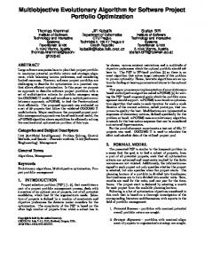
Our search from two independent runs yields two robust solutions, whose D/L ratios are both 0.013 at the operating condition of M∞=0.5. In comparison, the optimum found using a deterministic formulation has a D/L ratio of 0.0114. The D/L ratios for the final designs across the range M∞ ∈ [0.45, 0.55] attained by the traditional GA and max-min SAEA are summarized in Fig. 10. The traditional GA optimizes the 24 design variables to attain a lowest possible drag-to-lift ratio profile at M∞=0.5, irrespective of how the optimized design fares at other Mach numbers. Naturally, the optimum D/L=0.011 at M∞=0.5 is a reduction of 15% over the robust designs at the same Mach number. The penalty for this is the extreme sensitivity to changes in Mach number, where a slight change of ±0.02 (4%) about M∞=0.5 will result in roughly 50% jump in D/L. Moreover, the discontinuity in D/L is undesirable from viewpoint of aircraft stability. On the other hand, even though the robust solutions have a higher D/L ratio of 0.013 at M∞=0.5, the results in Fig. 10 indicate that the max-min SAEA achieves a better overall drag reduction across the entire design range, with an average D/L value of 0.013 versus 0.014 of the traditional GA. In this particular case, the robust GA achieves a 7% average-drag reduction over the entire interval with respect to the traditional GA. Moreover, transition of D/L from lower to higher Mach values is smooth. Hence it can be concluded that the robust scheme results in superior designs for low computational effort. It is also worth noting that the final designs are quite different for the traditional GA and max-min SAEA. This is evident in Figures 11 and 12, which compare the shapes and pressure profiles of the three solutions.
Paper Submitted to IEEE TEC
28
E. Performance Validation of Final Designs
To verify that unconstrained optimization of D/L in this study has not led to degradation in L, we now compare the lift, drag and pitching-moment profiles of the final designs. Fig. 13 shows the polars (L versus D graphs) of the various airfoils at the design speed Mach 0.5, and for AoA ranging from -4° to 9°. It can be seen that for the design point of AoA=2°, all four designs have high lift and lower drag compared to the baseline airfoil. At higher AoA all four designs offer better lift performance than the baseline geometry. It is interesting to note that, for a fixed value of L, the Category III designs (robust to change in Mach number) have lower drag than the baseline over the entire range of AoA, whereas the Category II design (robust to manufacturing errors) and the deterministic optimum actually underperform at negative AoA. Additionally, the lift and pitching moments are plotted in Fig. 14, where it can be seen that the deterministic and Category II designs perform generally better than the Category III designs in terms of lift performance. Finally, the pitching moments differ little from that of the baseline airfoil. In particular, the moments are negative for positive AoA, confirming that the designed airfoils are statically stable. VI. CONCLUSIONS In this paper, we presented a max-min surrogate-assisted EA for robust engineering design. The fundamental idea was to search for designs that have the best worst-case performance in the presence of parameter uncertainty. Further, by leveraging a trustregion approach which uses computationally cheap surrogate models, the present approach allows for the possibility of achieving robust design solutions on a limited computational budget.
Paper Submitted to IEEE TEC
29
The proposed algorithm was successfully applied to aerodynamic design of airfoil geometries that are robust to uncertainties in the operating conditions and manufacturing errors. It was shown that the present approach gives robust solutions that can be considered to be superior to those obtained using a deterministic optimization formulation. ACKNOWLEDGMENT The authors would like to thank the Parallel and Distributed Computing Centre at the School of Computer Engineering, Nanyang Technological University for providing support and computing resources to this work. REFERENCES [1] P. Hajela, J. Lee., “Genetic algorithms in multidisciplinary rotor blade design”,
Proceedings of 36th AIAA/ASME/ASCE/AHS/ASC Structures, Structural Dynamics and Material Conference, New Orleans, pp. 2187-2197, 1995. [2] Y. S. Ong and A.J. Keane, “Meta-Lamarckian in Memetic Algorithm”, IEEE Trans.
Evolutionary Computation, Vol. 8, No. 2, pp. 99-110, April 2004. [3] I. C. Parmee., D. Cvetkovi., A. H. Watson, C. R. Bonham, “Multi objective
satisfaction within an interactive evolutionary design environment”, Evolutionary Computation, Vol. 8, No. 2, pp. 197-222, 2000. [4] P. B. Nair and A. J. Keane,
“Passive Vibration Suppression of Flexible Space
Structures via Optimal Geometric Redesign”, AIAA Journal, Vol. 39, No. 7, pp. 1338-1346, 2001.
Paper Submitted to IEEE TEC
30
[5] L. Huyse, “Solving Problems of Optimisation Under Uncertainty as Statistical
Decision Problems”, AIAA-2002-1519, 2001. [6] W. Chen and J. K. Allen and K.-L. Tsui and F. Mistree. “A procedure for robust
design: Minimizing variations caused by noise factors and control factors,’’ ASME Journal of Mechanical Design, Vol. 118, pp. 478-485, 1996. [7] J. Branke. “Creating robust solutions be means of evolutionary algorithms,’’ Parallel
Problem Solving from Nature, pp. 119-128, 1998. [8] T. Ray. “Constrained robust optimal design using a multi-objective evolutionary
algorithm,’’ Proceedings of the Congress on Evolutionary Computation, pp. 419-424, 2002. [9] Y. Jin and B. Sendhoff. “Trade-off between performance and robustness: An
evolutionary multiobjective approach,’’ Proceedings of the Second International Conference on Evolutionary Multi-criterion Optimization, pp. 237-251, 2003. [10] S. Tsutsui and A. Ghosh , “Genetic Algorithms with a Robust Solution Searching
Scheme”, IEEE Trans. Evolutionary Computation, Vol. 1, No. 3, pp. 201-208, 1997. [11] S. Tsutsui and A. Ghosh, “A Comparative Study on the Effects of Adding
Perturbations to Phenotypic Parameters in Genetic Algorithm with a Robust Solution Searching Scheme”, IEEE Systems, Man, and Cybernetics Conference, pp. 585-591, 1999. [12] D. V. Arnold and H. G. Beyer, “Local Performance of the (1+1)-ES in a Noisy
Environment”, IEEE Trans. Evolutionary Computation, Vol. 6, No. 1. , pp. 30-41, 2002.
Paper Submitted to IEEE TEC
31
[13] D. Wiesmann, U. Hammel and T. Back, “Robust design of multilayer optical
coatings by means of evolutionary algorithms”, IEEE Trans. Evolutionary Computation, Vol. 2, No 4, pp 162-167, 1998. [14] D. K. Anthony and A. J. Keane, “Robust-Optimal Design of a Lightweight Space
Structure Using a Genetic Algorithm”, AIAA Journal, Vol. 41, No. 8, pp. 1601-1604, 2003. [15] J. M. Fitzpatrick and J. J. Grefenstette, “Genetic algorithms in noisy environments”,
Machine Learning, No. 3, pp. 101-120, 1988. [16] U. Hammel and T. Back, “Evolution Strategies on Noisy Functions: How to Improve
Convergence Properties”, Parallel Problem Solving from Nature - PPSN III, Y. Davidor H.-P. Schwefel and R. Manner (Eds.), Springer, Berlin, pp. 159-168, 1994. [17] B. L. Miller and D. E. Goldberg, “Genetic Algorithms, Selection Scheme, and the
Varying Effect of Noise”, Evolutionary Computation, Vol. 4, No. 2, pp. 113-131, 1996. [18] J. Branke, “Evolutionary Optimization in Dynamic Environments”, Kluwer Academic
Publishers, 2002. [19] Y. Jin and J. Branke, “Evolutionary Optimization in uncertain environments – A
survey”, IEEE Trans. Evolutionary Computation, Vol. 9, No. 3, 2005. [20] Y. Ben-Haim and I. Elishakoff, Convex Models of Uncertainty in Applied
Mechanics, Elsevier Science Publishers, Amsterdam, The Netherlands, 1990. [21] A. Wald, Statistical Decision Functions, Wiley, New York 1950. [22] A. J. Keane and P. B. Nair, Computational Approaches to Aerospace Design, John-
Wiley and Sons, 2005.
Paper Submitted to IEEE TEC
32
[23] K.-H. Liang, X. Yao, and C. Newton, “Evolutionary Search of Approximated N-
Dimensional Landscape”, International Journal of Knowledge-based Intelligent Engineering Systems, Vol. 4, No. 3, pp. 172-183, 2000. [24] Y. Jin, M. Olhofer and B. Sendhoff, “A Framework for Evolutionary Optimization
with Approximate Fitness Functions”, IEEE Trans. Evolutionary Computation, Vol. 6, No. 5, pp. 481-494, 2002. [25] Y. S. Ong, P. B. Nair and A. J. Keane, “Evolutionary Optimization of
Computationally Expensive Problems via Surrogate Modeling”, AIAA Journal, Vol. 41, No. 4, pp. 687-696, 2003. [26] Y. Jin, “A comprehensive survey of fitness approximation in evolutionary
computation”, Soft Computing Journal, 9(1): 3-12, 2005. [27] Z. Z. Zhou, Y. S. Ong and P. B. Nair, “Hierarchical Surrogate-Assisted Evolutionary
Optimization Framework”, IEEE Congress on Evolutionary Computation, June 2023, 2004. [28] Y. S. Ong, P. B. Nair, A. J. Keane and K. W. Wong, “Surrogate-Assisted
Evolutionary Optimization Frameworks for High-Fidelity Engineering Design Problems”, Knowledge Incorporation in Evolutionary Computation, editor: Y. Jin, Studies in Fuzziness and Soft Computing Series, Springer Verlag, 2004. [29] Z. Z. Zhou, Y. S. Ong, P. B. Nair, A. J. Keane and K.Y. Lum, “Combining global
and local surrogate models to accelerate evolutionary optimization”, IEEE Trans. Systems, Man, and Cybernetics – Part C, in press, 2005. [30] L. Kocis and W.J. Withen, ‘‘Computational investigations of low-discrepancy
sequences,’’ ACM Transactions on Mathematical Software, 23(2), 1997, pp. 266-294.
Paper Submitted to IEEE TEC
33
[31] C. Bishop, “Neural Networks for Pattern Recognition”, Oxford University Press,
1995. [32] I. Elishakoff, R.T. Haftka and J. Fang, “Structural optimization under bounded
uncertainty – optimization with anti-optimization,” Computers and Structures, Vol. 53, No. 6, pp. 1401-1405, 1994. [33] R.M. Hicks and P.A. Henne, “Wing design by numerical optimization”, Journal of
Aircraft, Vol. 15, No. 7, pp. 407-412, 1978. [34] S. Obayashi and T. Tsukahara, “Comparison of Optimization Algorithms for
Aerodynamic Shape Design”, AIAA Journal, Vol. 35, No. 8, pp. 1411-1412, 1997. [35] A. Jameson, “Aerodynamic design via control theory”, Journal of Scientific
Computing, Vol. 3, No. 3, pp. 233-260, 1988. [36] D. Quagliarella and A.D. Cioppa, “Genetic Algorithms Applied to the Aerodynamic
Design of Transonic Airfoils”, Journal of Aircraft, Vol. 32, No. 4, pp. 889-891, 1995. [37] N. Marco, S. Lanter, J.-A. Desideri, B. Mantel and J. Periaux, “Parallelized genetic
algorithm for a two dimensional-shape optimum design problem”, Surveys on Mathematics for Industry, Vol. 9, No. 3, pp. 207-221, 2000. [38] A. Hacioglu and I. Ozkol, “Transonic airfoil design and optimization by using
vibrational genetic algorithm”, Aircraft Engineering and Aerospace Technology, Vo. 75, No. 4, pp. 350-357, 2003. [39] K.C. Giannakoglou, “Design of optimal aerodynamic shapes using stochastic
optimization methods and computational intelligence”, Progress in Aerospace Sciences, Vol. 38, No. 1, pp. 43-76, 2002.
Paper Submitted to IEEE TEC
34
[40] L. Huyse, S.L. Padula and W. Li, “Probabilistic approach to free-form airfoil shape
optimization under uncertainty”, AIAA Journal, Vol. 40, No. 9, pp. 1764-1772, 2002. [41] W. Li, L. Huyse and S. Padula, “Robust airfoil optimization to achieve drag
reduction over a range of Mach number”, Structural and Multidisciplinary Optimization, Vol. 24, No. 1, pp. 38-50, 2002. [42] M. Drela, “Pros & Cons of Airfoil Optimization”, In D.A. Caughey and M.M. Hafez
(eds.), Frontiers of Computational Fluid Dynamics, World Scientific, Singapore, 1998. [43] S. Peigin and B. Epstein, “Robust optimization of 2D airfoils driven by full Navier-
Stokes computation”, Computer & Fluids, Vol. 33, No. 9, pp. 1175-1200, 2004. th
[44] A.D. Jr. Anderson, Introduction to Flight, 4 edition, McGraw-Hill, 2000.
Paper submitted to IEEE TEC
35
TABLE I PARAMETERS USED FOR 2D SYNTHETIC FUNCTION IN (6). Centre / Peak Location Width parameter (σ) Multiplier (1,1)
0.3
0.7
(1,3)
0.4
0.75
(3,1) {Robust Solution}
1.0
1.0
(3,4) {Highest Peak}
0.4
1.2
(5,2)
0.6
1.0
TABLE II PARAMETERS USED FOR 5-DIMENSIONAL AND 10-DIMENSIONAL SYNTHETIC FUNCTIONS OF 10 PEAKS DERIVED FROM (5). Centre / Peak Location Centre / Peak Location Width Multiplier parameter (σ) (10, 1.0, 6.0, 7.0, 8.0) (1.0, 1.0, 6.0, 7.0, 8.0, 1.0, 1.0, 0.3 0.7 6.0, 7.0, 8.0) (1.0, 3.0, 8.0, 9.5, 2.0) (1.0, 3.0, 8.0, 9.5, 2.0, 1.0, 3.0, 0.4 0.75 8.0, 9.5, 2.0) (3.0, 1.0, 3.0, 2.0, 5.0) (3.0, 1.0, 3.0, 2.0, 5.0, 3.0, 1.0, 1.0 1.0 {Robust Solution} 3.0, 2.0, 5.0) (3.0, 4.0, 1.3, 5.0, 5.0) (3.0, 4.0, 1.3, 5.0, 5.0, 3.0, 4.0, 0.4 1.2 {Highest Peak} 1.3, 5.0, 5.0) (5.0, 2.0, 9.6, 7.3, 8.6) (5.0, 2.0, 9.6, 7.3, 8.6, 5.0, 2.0, 0.6 1.0 9.6, 7.3, 8.6) (7.5, 8.0, 9.0, 3.2, 4.6) (7.5, 8.0, 9.0, 3.2, 4.6, 7.5, 8.0, 0.5 0.6 9.0, 3.2, 4.6) (5.7, 9.3, 2.2, 8.4, 7.1) (5.7, 9.3, 2.2, 8.4, 7.1, 5.7, 9.3, 0.1 0.5 2.2, 8.4, 7.1) (5.5, 7.2, 5.8, 2.3, 4.5) (5.5, 7.2, 5.8, 2.3, 4.5, 5.5, 7.2, 1.0 0.2 5.8, 2.3, 4.5) (4.7, 3.2, 5.5, 7.1, 3.3) (4.7, 3.2, 5.5, 7.1, 3.3, 4.7, 3.2, 0.2 0.4 5.5, 7.1, 3.3) (9.7, 8.4, 0.6, 3.2, 8.5) (9.7, 8.4, 0.6, 3.2, 8.5, 9.7, 8.4, 0.3 0.1 0.6, 3.2, 8.5)
Paper submitted to IEEE TEC
36
TABLE III SUMMARY OF RESULTS OBTAINED USING GAS/RS3 ON THE TEST FUNCTIONS. GA/RS Method
Pure SEM Worst MEM m=3 Worst MEM m = 10 Worst MEM m = 20 Maxmin SAEA
Number of times arriving at the Most Robust Peak (Over 20 Independent Runs) 2D, 5 Peaks 5D, 10 Peaks 10D, 10 Peaks Average Average Average Convergence no. of Convergence no. of Convergence no. of exact exact exact function function function evaluation evaluation evaluation s s s 7 9,900 14 14,920 5 128,60 16
31,500
18
42,780
15
56,760
20
110,400
20
130,800
16
138,800
20
206,000
20
273,600
17
340,800
20
30,960
20
34,800
20
49,210
Paper submitted to IEEE TEC
37
BEGIN EA/RS Initialize: Generate a population of designs. While (termination condition is not satisfied) For (each individual xi in population) •
For (j =1 to m) Draw realization of uncertain parameters δ j from given distribution Perturb individual i to arrive at x ′j ← xi + δ j Evaluate fitness of perturbed solution f ( x ′j )
•
End For Determine effective fitness, F(xi), of individual i, 1 m F ( xi ) = ∑ j =1 f ( x ′j ) or F ( xi ) = worst{ f ( x1′), f ( x2′ ),..., f ( xm′ )} m
End For Apply standard EA operators to create a new population. End While END
Fig. 1. Evolutionary algorithm with robust solution searching schemes for category II uncertainty.
f (x1, x2)
x2 x1
Fig. 2. A plot of the 2D synthetic function in (6).
Paper submitted to IEEE TEC
38
Trust-Region Enabled Max-min SAEA BEGIN Initialize: Generate a database containing a population of designs. (Optional: upload a historical database if exists) While (EA termination condition is not satisfied) For (each individual i in population) If (Status is database building) Evaluate individual i using exact analysis code f ( x i ) Update vector x i and corresponding fitness value f ( x i ) in database Else { Apply trust-region enabled feasible SQP solver } o Set trust-region sub-problem, k =1, ∆ = δ While (trust-region termination condition not satisfied) Choose from database n nearest design points to the individual x ck
Construct a local RBF surrogate model using these points Establish the domain in which the uncertain parameters vary Ω Locate the point with worst-case fitness,
xlok , in direct
neighborhood of individual x ck (within bounds specified by the domain Ω ) using the RBF surrogate Evaluate xlok using exact analysis code Update
vector xlok and
corresponding
exact
fitness
value f ( x ) in the database k lo
Calculate the figure-of-merit, ρ defined in equation (12). k
Update trust region size ∆ ensuring that ∆ ∈ Ω Increment k by 1. End While Set F ( x i ) = f ( x lok ) , i.e., the fitness of individual i is set to the worstcase value k
End if Return F ( x i ) as the fitness of individual i End For Apply standard EA operators to create a new population. End While END
Fig. 3. Trust-Region enabled max-min SAEA
k
Paper submitted to IEEE TEC
f ( x ) = e − ( x −1) + 2.5e − ( x −1.8) + e − ( x − 3)
2
/ 0.5
+ 3.2 e − ( x −11)
2
2
/ 0.5
/ 0.02
+ 2 e − ( x −1.25)
/ 0.18
2
+ 2.5e − ( x − 2.2 )
+ 2e − ( x − 6) 2
39
2
/ 0.32
/ 0.045
2
/ 0.02
+ 0.5e − ( x −1.5) + 2 e − ( x − 2.4 )
+ 2.2 e ( x − 7 )
+ 1.2 e − ( x −12 )
2
2
/ 0.18
2
2
+ 2 e − ( x −1.6 )
/ 0.0128
/ 0.005
+ 2 e − ( x − 2.75)
+ 2.4 e − ( x − 8)
2
/ 0.5
2
2
/ 0.005
/ 0.045
+ 2.3e − ( x − 9.5)
2
/ 0.5
/ 0.18
Fig. 4. Illustration of effective fitness functions obtained using average and worst-case analysis for a model problem involving maximization of f ( x ) .
Paper submitted to IEEE TEC
40
lift L thrust T angle of attack α direction of flight
θ
drag D weight (a)
C (contour)
L n (σ ) (normal unit vector) p(σ ) (pressure)
AoA M∞
D
flow direction (b)
Fig. 5. Forces acting on: (a) an airplane, and (b) an airfoil
Paper submitted to IEEE TEC
41
Fig. 6. Airfoil geometry characterized using a 24-parameter Hicks-Henne representation (The bottom labels indicate the values of the 12 parameters ti)
Airfoil Shapes 0.1 0.08 0.06 0.04 0.02 0
Deterministic optimal design Robust to manufacturing errors
-0.02 -0.04 -0.06 -0.08
0
0.2
0.4 0.6 Normalized Chord
0.8
1
Fig. 7. Comparison of airfoil geometries obtained using traditional GA (deterministic design) and max-min SAEA (robustness to manufacturing errors).
Paper submitted to IEEE TEC
42
Upper and lower surface pressure coefficients 1.5 1 0.5 0 -0.5
Deterministic optimal design Robust to manufacturing errors
-1 -1.5
0
0.1
0.2
0.3
0.4 0.5 0.6 Normalized Chord
0.7
0.8
0.9
1
Fig. 8. Comparison of pressure profiles obtained using traditional GA (deterministic design) and max-min SAEA (robustness to manufacturing errors).
Fig. 9. Probability density function of D/L Ratio for deterministic and robust designs using Monte Carlo simulation.
Paper submitted to IEEE TEC
43
Mach vs Drag/Lift (D/L)
0.02
D/L
0.015 0.01
Deterministic Design Robust Design 1 Robust Design 2
0.005
0. 45 0. 45 8 0. 46 6 0. 47 4 0. 48 2 0. 49 0. 49 8 0. 50 6 0. 51 4 0. 52 2 0. 53 0. 53 8 0. 54 6
0
Mach
Fig. 10. The relationship between Mach and D/L for deterministic and robust designs using traditional GA and Max-min SAEA, respectively.
Fig. 11. Comparison of airfoil geometries obtained using traditional GA (deterministic design) and max-min SAEA (designs 1 and 2, robustness to changing Mach number).
Paper submitted to IEEE TEC
44
Upper and lower surface pressure coefficients 1.5 1 0.5 0 -0.5
Deterministic optimal design Robust to Mach changes (design 1) Robust to Mach changes (design 2)
-1 -1.5
0
0.1
0.2
0.3
0.4 0.5 0.6 Normalized Chord
0.7
0.8
0.9
1
Fig. 12. Comparison of pressure profiles obtained using traditional GA (deterministic design) and max-min SAEA (designs 1 and 2, robustness to changing Mach number).
Paper submitted to IEEE TEC
45
Polars (L vs D graphs) of Final Designs at Mach 0.5
1 0.8
AoA = 9 deg
0.6
increasing AoA
0.2
Design Point: AoA = 2 deg
0
Baseline NACA 0015 Robust to Mach changes (design 1) Robust to Mach changes (design 2) Robust to manufacturing errors Deterministic optimal design
-0.2 -0.4 -0.6
AoA = -4 deg 0
1
0.005
0.01
0.015
0.02
0.03
0.035
0.04
Lift and Pitching Moment of Final Designs at Mach 0.5
0.8
Lift
0.025
Drag (D) Fig. 13. Polars (L vs. D graphs) of final designs at Mach 0.5
0.045
-1 -0.8
Lift
0.6
-0.6
0.4
-0.4
Pitching Moment 0.2
-0.2
0
0
Baseline NACA 0015 Robust to Mach changes (design 1) Robust to Mach changes (design 2) Robust to manufacturing errors Deterministic optimal design
-0.2 -0.4 -0.6 -4
-2
0
2
4
6
AoA (deg.) Fig. 14. Lift and pitching moment of final designs at Mach 0.5
8
0.2 0.4
10
0.6
Pitching Moment
Lift (L)
0.4