Maximum Likelihood Joint Channel and Data Estimation Using ...

IEEE TRANSACTIONS ON SIGNAL PROCESSING, VOL. 46, NO. 5, MAY 1998

[12] F. Khalil, J. P. Jullien, and A. Gilloire, “Microphone array for sound pickup in teleconference systems,” J. Audio Eng. Soc., vol. 42, no. 9, pp. 691–700, Sept. 1994. [13] T. Chou, “Frequency-independent beamformer with low response error,” in Proc. IEEE Int. Conf. Acoust., Speech, Signal Process. (ICASSP), Detroit, MI, May 1995, pp. 2995–2998. [14] D. B. Ward, R. A. Kennedy, and R. C. Williamson, “FIR filter design for frequency-invariant beamformers,” IEEE Signal Processing Lett., vol. 3, pp. 69–71, Mar. 1996.

Maximum Likelihood Joint Channel and Data Estimation Using Genetic Algorithms S. Chen and Y. Wu

Abstract— A batch blind equalization scheme is developed based on maximum likelihood joint channel and data estimation. In this scheme, the joint maximum likelihood optimization is decomposed into a twolevel optimization loop. A micro genetic algorithm is employed at the upper level to identify the unknown channel model, and the Viterbi algorithm is used at the lower level to provide the maximum likelihood sequence estimation of the transmitted data sequence. As is demonstrated in simulation, the proposed method is much more accurate compared with existing algorithms for joint channel and data estimation. Index Terms—Blind equalization, genetic algorithms, maximum likelihood estimation.

1469

This algorithm may be viewed as an “enhanced” Viterbi algorithm (VA) that retains several surviving sequences and associated channel estimates for each state of the trellis. The quantized channel algorithm [11] is a batch procedure that maintains a family of candidate channels with discrete parameters. Each channel model is used by the VA to decode data, and the algorithm selects the most likely quantized channel. In this correspondence, we propose a novel scheme for joint channel and data estimation using genetic algorithms (GA’s) [13]–[16]. We develop a two-layer strategy for joint optimization over channel and data by combining the GA with the VA. At the top layer, an efficient version of GA known as the micro-GA (GA) [15] searches the channel parameter space to optimize the ML criterion. The bottom layer consists of a number of VA units: one for each member of the channel population. Each VA unit decodes data based on the given channel model and feeds back the corresponding likelihood metric value to the GA. The performance of this GA scheme is investigated in a simulation study. The results obtained clearly demonstrate that the GA-based scheme has superior performance over other existing methods for joint channel and data estimation. II. MAXIMUM LIKELIHOOD BLIND EQUALIZATION Throughout this study, the channel is modeled as a finite impulse response filter with an additive noise source [17]. Specifically, the received signal at sample k is given by

r(k) = I. INTRODUCTION Since the pioneering work of Sato [1], three families of blind equalization techniques have emerged. The first family of blind adaptive algorithms, which is commonly known as Bussgang algorithms, constructs a transversal equalizer directly to unravel the effects of the channel impulse response [1]–[4]. This class of blind equalizers has very low computational complexity but suffers from the drawback of slow convergence. The second family of blind equalization algorithms is based on higher order cumulants [5]–[8]. This second class of blind equalizers, although very general and powerful, requires a large amount of received data samples and extensive computation to estimate higher order cumulants. The third family of blind adaptive algorithms uses some blind approximations of the maximum likelihood sequence estimation (MLSE) to perform a joint channel and data estimation [9]–[12]. The resulting blind equalizers are therefore computationally very expensive. A major advantage of this third approach is that relatively few signal samples are required to achieve the equalization objective. When both the channel and transmitted data sequence are unknown, in theory, their optimal estimates can be obtained via the maximum likelihood (ML) optimization over channel and data jointly. The computational requirement of such a joint optimization procedure is, however, prohibitively large. In practice, approximations are adopted. A straightforward way is to employ a batch iterative process between data decoding and channel estimation [9]. Seshadri [10] presented a recursive algorithm for joint channel and data estimation. Manuscript received October 22, 1996; revised September 16, 1997. The associate editor coordinating the review of this paper and approving it for publication was Dr. Ali H. Sayed. The authors are with the Department of Electrical and Electronic Engineering, University of Portsmouth, Portsmouth, U.K. Publisher Item Identifier S 1053-587X(98)03267-X.

n

01

i=0

ai s(k 0 i) + e(k)

(1)

where

na channel length; ai channel taps; e(k) Gaussian white noise with zero mean and variance e2 ; and the symbol sequence fs(k)g is independently identically distributed with a variance s2 . We will assume that the multilevel pulse amplitude modulation (M -PAM) scheme is used. The signal-to-noise ratio (SNR) of the system is defined as SNR = s2

n

01

i=0

a2i =e2 :

(2)

Joint channel and data estimation can be performed based on the ML criterion. Let

r = [r(1)r(2) 1 1 1 r(N )]T s = [s(0na + 2) 1 1 1 s(0)s(1) 1 1 1 s(N )]T a = [a0 a1 1 1 1 an 01 ]T

(3)

be the vector of N received data samples, the transmitted data sequence, and the vector of channel taps, respectively. The probability density function of the received data vector r conditioned on the channel impulse response a and the symbol vector s is

p(rja; s) =

1 N=2 (2e2 )

1 exp 0 21 2

N

e k=1

r(k) 0

n

01

i=0

ai s(k 0 i)

2

:

(4)

The joint ML estimate of a and s is obtained by maximizing p(rja; s) over a and s jointly. Equivalently, the ML solution is the minimum

1053–587X/98$10.00  1998 IEEE

1470

IEEE TRANSACTIONS ON SIGNAL PROCESSING, VOL. 46, NO. 5, MAY 1998

of the cost function

J (a; s) =

N

k=1

r(k) 0

n

01

i=0

2

ai s(k 0 i)

(5)

over a and s, that is

3 ; s3 ) = arg

(a

min J (a; s)

a; s

:

(6)

Two special cases of the ML solution (a3 ; s3 ) are well known. When a training sequence is available, the ML estimate of the channel a is the usual least squares solution. The MLSE for the data sequence s when the channel is known can be obtained using the standard VA. When neither a nor s are known, in theory, the joint ML estimate 3 3 (a ; s ) can be obtained. However, such an optimal solution is too expensive to compute, except for the simplest case. In practice, suboptimal solutions are adopted for computational purposes. The algorithm based on a blind trellis search technique [10] is such an example. In the standard VA with the known channel, one surviving sequence is retained for each state of the trellis. When the channel is unknown, an enhanced VA is adopted that retains m > 1 surviving sequences for each state of the trellis. Each of these m surviving sequences is used to adapt a channel model. This enhanced VA decoding and m-channel estimation process can be implemented recursively. The joint minimization process (6) can also be performed using an iterative loop first over the data sequences s and then over all the possible channels a

3 ; s3 ) = arg

(a

min min J (a; s)

a

s

:

(7)

The inner optimization can be carried out using the VA. In order to obtain the true optimal solution, the outer optimization must be performed over all the possible channels a, the complexity of which is generally prohibitive. Suboptimal solutions are usually sought by constraining the search to a finite set. For example, the quantized channel algorithm [11] uses a family of 2n quantized channels. GA’s are natural choices for performing the outer optimization in (7) since they can search the channel space efficiently with a finite population. III. GENETIC ALGORITHMS The first step in applying GA’s is to encode the parameters to be optimized. We use the popular binary encoding scheme [13]. A simple GA usually consists of three operations, namely, selection, crossover, and mutation [14], at each cycle. An “elitist” strategy [16], which automatically copies a few of the best solutions in the population into the next generation, is often incorporated. Two commonly used methods of selection are the proportional and tournament selections [14], [15]. In the crossover operation, we adopt multiple crossover points [14], and the number of crossover points in our application is equal to the number of the parameters. For many engineering problems, the goal is to find a global optimum solution as quickly as possible rather than a good average performance of potential solutions. For this purpose, the so-called GA [15] seems to offer certain advantages. The population size used in a GA is much smaller than that used in “standard” versions of GA. Simply adopting a very small population size and letting the search converge just once, however, is not very useful apart from quickly allocating some local optimum. Therefore, in a GA, after the search has converged, the population is reinitialized with random values, whereas the best individual found up to that point is automatically copied to the newly generated population. The reinitialization is repeated until no further improvement can be achieved.

A population size of five was suggested in [15] for the GA. Generally speaking, however, the more complex the search space is, the larger the population size should be. An appropriate population size also depends on the application problem. In our application, the population size np is given by np = 5 2 na , where na is the channel length. This is still considerably smaller than a typical population size used by standard GA’s. In our GA implementation, the crossover rate is set to 1.0 to facilitate a high rate of information exchange, whereas the mutation rate is set to 0.0 (no mutation) as the reinitialization of the population will keep the diversity of potential solutions fairly well. Another consequence of small population size is the method of selection. Due to the small population size of GA, the law of averages does not hold well, and the tournament selection is used in choosing parents for reproduction. IV. GAS FOR JOINT CHANNEL AND DATA ESTIMATION The proposed scheme, consisting of a GA and np VA units, involves an initialization phase and two loops. In the initialization, n ^ i gi=1 is randomly chosen, and the best a set of channel models fa ^Rec is randomly selected from channel vector found up to that point a the initial population. It is assumed that each channel model in the population is normalized according to n

01 a2 = 1:0:

(8)

i

i=0

01 a2 )2 can always This is realistic since the channel energy ( n i s i=0 2 be estimated, and s is known. The search range for each parameter is, therefore, (01; 1). The inner loop of the GA-based scheme is summarized as follows. Step 1) For 1  i  np , the ith VA unit decodes data based on ^ i and feeds back the likelihood metric, which is given a ^i . the fitness function value fi corresponding to a Step 2) Let fbest be the best fitness value of the current popula^ best . tion, and let the corresponding channel model be a If n

i=1

(fbest

0 f ) < f i

best

(9)

the inner loop is terminated, where  is a predefined small n ^i gi=1 positive constant. Otherwise, a new generation of fa is produced, and the algorithm goes back to Step 1. After the convergence of the inner loop, the convergence of the overall process is tested. If

ka^

best

p 0 a^ k <  4n Rec

a

(10)

the outer loop is terminated, p where the small positive scalar  defines the search accuracy, and 4na is the Euclidean norm of the search space [as the search range for each parameter is (01; 1)]. Otherwise, ^ Rec is reset to a ^ Rec = a ^ best , and the population is reinitialized, a the inner loop restarts. It is possible that a reinitialization of the population may sample the same regions of the search space as the previous population did. To increase the chance of converging to a global optimum, the outer loop test can be amended as follows: The overall process has converged only if the test (10) has been satisfied for several consecutive times. Convergence properties of the proposed GA scheme are extremely difficult to analyze due to the highly complex nature of the underlying optimization problem (7). Since GA’s are global optimization techniques, our method is more likely to find a global optimal solution than the methods of [9] and [11]. Strictly speaking, it can only be said that on average, the GA converges to a global

IEEE TRANSACTIONS ON SIGNAL PROCESSING, VOL. 46, NO. 5, MAY 1998

optimum because of the probabilistic nature of the GA. It does not guarantee that, for any particular realization of the noisy signal r and any particular run of the GA, convergence to an optimal solution of the ML joint channel and data estimation can always be ensured. In our simulation study, however, we have not encountered a nonconvergent case. Let CVA be the complexity of the VA required to decode a data sequence of N samples, and let NVA be the total number of VA calls required for the GA algorithm to converge. The complexity of the GA-based scheme is obviously NVA 2 CVA . This is considerably more than Seshadri’s algorithm. Our experimental results suggest that a population size np of around 5 2 na for the GA implementation, rather than np = 5, is appropriate for our application. This population size is smaller than that used by the quantized channel algorithm [11]. For 2-PAM problems, the quantized channel algorithm requires a family of 2n channel models. A straightforward application of the quantized channel algorithm to M -PAM problems would require a family of M n channel models, which would be impractical to compute for high-order M . Therefore, a reduced constellation approach has to be adopted in order to maintain a family of 2n channel models. Our GA-based method does not need to adopt a reduced constellation approach.

1471

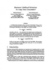
Fig. 1. Mean tap error as a function of VA evaluations averaged over 100 = 50. different runs. Channel 1, 2-PAM and the number of data samples

N

V. SIMULATION STUDY Computer simulation was conducted to test the proposed GA scheme using three channels taken from [17]. The impulse response of these three channels is given by Channel 1 Channel 2 Channel 3

Fig. 2. Mean tap error as a function of VA evaluations averaged over 100 = 100. different runs. Channel 1, 8-PAM and the number of data samples

N

a = [0:407 0:815 0:407]T

a = [00:21 00:50 0:72 0:36 0:21]T

a = [0:227 0:460 0:688 0:460 0:227]T

(11)

respectively. In practice, the performance of the algorithm can only be observed through the best estimated mean square error (MSE) defined by MSE =

1

N

r(k) 0

n 01

a~i s~(k 0 i)

2

(12)

N k=1 i=0 ^best = [~ a0 a~1 1 1 1 a~n 01 ]T is the most likely channel model where a s(0na + 2) 1 1 1 s~(1) 1 1 1 s~(N )]T is the in the population, and ~s = [~

Fig. 3. Mean tap error as a function of VA evaluations averaged over 100 different runs. Channel 2, 2-PAM and the number of data samples = 100.

N

^ best . In simulation, the performance ML sequence associated with a of the algorithm can also be assessed by the mean tap error (MTE)

2 ^best 0 ak : MTE = k 6 a

(13)

^ best converges to 0a. Otherwise, a ^best is ^best is used if a In (13), 0a used. This is necessary as the most likely channel model can converge to either a or 0a. Figs. 1–6 depict the MTE performance versus the number of VA evaluations for the three channels in (11) with 2-PAM and 8-PAM symbols and different noise levels, respectively. These results were obtained assuming the correct channel length na and were averaged over 100 different runs. Compared with the results of using the quantized channel algorithm given in [11], our GA scheme required a smaller number of VA evaluations to achieve a same level of MTE performance. The final results obtained by the GA method were also more accurate, particularly for high-order PAM. Table I shows the means and variances of the MSE and MTE over 100 runs for channel 1. The convergence of our GA scheme is consistent, as is evident from the very small variances of the MSE and MTE. Seshadri’s algorithm [10] is regarded as one of the best methods for joint channel and data estimation. A performance comparison between our GA method and Seshadri’s algorithm is not

Fig. 4. Mean tap error as a function of VA evaluations averaged over 100 different runs. Channel 2, 8-PAM and the number of data samples = 300.

N

straightforward as the former is a batch algorithm and the latter a recursive algorithm. Nevertheless, we compare the accuracy of the two methods. Tables II and III summarize the MTE performance and the number of received data samples used for the two methods. The results of Seshadri’s algorithm were estimated from the graphs in [10], which were also obtained by averaging over 100 runs. Our GA method is clearly much more accurate, particularly for high-

1472

IEEE TRANSACTIONS ON SIGNAL PROCESSING, VOL. 46, NO. 5, MAY 1998

Fig. 5. Mean tap error as a function of VA evaluations averaged over 100 = 100. different runs. Channel 3, 2-PAM and the number of data samples

N

Fig. 6. Mean tap error as a function of VA evaluations averaged over 100 = 200. different runs. Channel 3, 8-PAM and the number of data samples

N

TABLE I

RESULTS (MEANS

6 VARIANCES) FOR CHANNEL 1 AVERAGED OVER 100 RUNS

Fig. 7. Mean square error as a function of estimated channel length averaged over 100 different runs. Channel 1, 4-PAM and the number of data samples = 100.

N

Fig. 8. Mean square error as a function of estimated channel length averaged over 100 different runs. Channel 2, 2-PAM and the number of data samples = 100.

N

versus the estimated channel length. As expected, when the estimated channel length is correct, the MSE curve achieves the minimum. VI. CONCLUSIONS

TABLE II PERFORMANCE COMPARISON. 2-PAM

AND

SNR = 10 dB

TABLE III PERFORMANCE COMPARISON. 8-PAM

AND

SNR = 30 dB

order PAM. This advantage is, of course, obtained at the cost of computational complexity. In reality the channel length is unknown and has to be estimated. A simple and effective solution is to run the GA method with a set of different lengths. It is obvious that if the channel length used by the GA scheme is the true channel length, the MSE provided by the algorithm will reach a minimum value. In this way, the correct channel length can be identified. Figs. 7 and 8 illustrate the MSE

A batch method using the GA has been developed for blind equalization based on the ML joint channel and data estimation. Compared with other batch-type methods, such as the quantized channel approach, the GA-based scheme is more accurate and computationally more efficient in terms of the total number of required VA evaluations. Our simulation study has demonstrated that the GA-based scheme requires less received data samples to achieve much more accurate blind equalization results at the expense of computational complexity, compared with the best recursive blind trellis search technique. Simulation results have also shown that our GA-based method converges consistently with very small estimation variances. REFERENCES [1] Y. Sato, “A method of self-recovering equalization for multilevel amplitude-modulation systems,” IEEE Trans. Commun., vol. COMM-23, pp. 679–682, 1975. [2] D. Godard, “Self-recovering equalization and carrier tracking in twodimensional data communication systems,” IEEE Trans. Commun., vol. COMM-28, pp. 1867–1875, 1980. [3] J. R. Treichler and B. G. Agee, “A new approach to multipath correction of constant modulus signals,” IEEE Trans. Acoust., Speech, Signal Processing, vol. ASSP-31, pp. 459–472, Apr. 1983. [4] G. Picchi and G. Prati, “Blind equalization and carrier recovering using a stop-and-go decision-directed algorithm,” IEEE Trans. Commun., vol. COMM-35, pp. 877–887, 1987. [5] K. S. Lii and M. Rosenblatt, “Deconvolution and estimation of transfer function phase and coefficients for non-Gaussian linear processes,” Ann. Statist., vol. 10, pp. 1195–1208, 1982. [6] H.-H. Chiang and C. L. Nikias, “Adaptive deconvolution and identification of nonminimum phase FIR systems based on cumulants,” IEEE Trans. Automat. Contr., vol. 35, pp. 36–47, 1990.

IEEE TRANSACTIONS ON SIGNAL PROCESSING, VOL. 46, NO. 5, MAY 1998

[7] D. Hatzinakos and C. L. Nikias, “Blind equalization using a tricepstrumbased algorithm,” IEEE Trans. Commun., vol. 39, pp. 669–682, May 1991. [8] F.-C. Zheng, S. McLaughlin, and B. Mulgrew, “Blind equalization of nonminimum phase channels: Higher order cumulant based algorithm,” IEEE Trans. Signal Processing, vol. 41, pp. 681–691, Feb. 1993. [9] M. Ghosh and C. L. Weber, “Maximum-likelihood blind equalization,” in Proc. SPIE, San Diego, CA, 1991, vol. 1565, pp. 188–195. [10] N. Seshadri, “Joint data and channel estimation using blind trellis search techniques,” IEEE Trans. Commun., vol. 42, pp. 1000–1011, Feb./Mar./Apr. 1994. [11] E. Zervas, J. Proakis, and V. Eyuboglu, “A quantized channel approach to blind equalization,” in Proc. ICC, Chicago, IL, 1992, vol. 3, pp. 351.8.1–351.8.5.

1473

[12] J. G. Proakis, “Adaptive algorithms for blind channel equalization,” in Proc. 3rd IMA Conf. Math. Signal Process., Univ. Warwick, Warwick, U.K., 1992. [13] J. H. Holland, Adaptation in Natural and Artificial Systems. Ann Arbor, MI: Univ. Michigan Press, 1975. [14] D. E. Goldberg, Genetic Algorithms in Search, Optimization, and Machine Learning. Reading, MA: Addison-Wesley, 1989. [15] K. Krishnakumar, “Micro-genetic algorithms for stationary and nonstationary function optimization,” in Proc. SPIE Intell. Cont. Adapt. Syst., 1989, vol. 1196, pp. 289–296. [16] L. Yao and W. A. Sethares, “Nonlinear parameter estimation via the genetic algorithm,” IEEE Trans. Signal Processing, vol. 42, pp. 927–935, Apr. 1994. [17] J. G. Proakis, Digital Communications. New York: McGraw-Hill, 1983.