Statistica Sinica 21 (2011), 107-128
MAXIMUM LOCAL PARTIAL LIKELIHOOD ESTIMATORS FOR THE COUNTING PROCESS INTENSITY FUNCTION AND ITS DERIVATIVES Feng Chen University of New South Wales
Abstract: We propose estimators for the counting process intensity function and its derivatives by maximizing the local partial likelihood. We prove the consistency and asymptotic normality of the proposed estimators. In addition to the computational ease, a nice feature of the proposed estimators is the automatic boundary bias correction property. We also discuss the choice of the tuning parameters in the definition of the estimators. An effective and easy-to-calculate data-driven bandwidth selector is proposed. A small simulation experiment is carried out to assess the performance of the proposed bandwidth selector and the estimators. Key words and phrases: Asymptotic normality, automatic boundary correction, composite likelihood estimator, consistency, counting process, intensity function, local likelihood, local polynomial methods, martingale, maximum likelihood estimator, multiplicative intensity model, partial likelihood, point process, Z-estimator.
1. Introduction The counting process is a useful statistical model that is extensively applied in the analysis of data arising from such fields as medicine and public health, biology, finance, insurance, and social sciences. The evolution of a counting process over time is (stochastically) governed by its intensity process, and by its intensity function in the case of multiplicative intensity process models. Therefore, to understand the behavior of a multiplicative intensity counting process, the estimation of the intensity function is an important question. There is a sizable literature devoted to this question. Ramlau-Hansen (1983) applied the kernel smoothing method to estimate the intensity function and established the consistency and local asymptotic normality of the proposed estimator. RamlauHansen also proposed to estimate the derivatives of the intensity function by differentiating the estimator of the intensity function. Karr (1987) used the sieve method and established the strong consistency and the asymptotic normality of the resultant estimator for the intensity function. Antoniadis (1989) proposed a penalized maximum likelihood estimator for the intensity function and proved its consistency and asymptotic normality. Patil and Wood (2004) used the wavelet
108
FENG CHEN
method to estimate the intensity function and calculated the mean integrated squared error of the estimator. Chen et al. (2008) proposed to estimate the intensity function and its derivatives using a local polynomial estimator based on martingale estimating equations, and proved the consistency and asymptotic normality of the estimators. The roughness penalty method and the sieve method are computationally expensive because of the potentially high dimensional optimization involved. Also, formal methods for derivative estimation based on these methods or the wavelet thresholding method seem lacking. The kernel smoothing method is computationally very appealing, but requires extra effort in modifying the estimators for boundary points to reduce the boundary or edge effects. The biased martingale estimating equation method of Chen et al. (2008) provides estimators for the intensity function and its derivatives in a unified manner and enjoys both the computational ease and the automatic boundary correction property of local polynomial type methods (Chen, Yip, and Lam (2009)) but, from a theoretic point of view, the construction of the estimating equations is somewhat arbitrary. In this paper we propose an estimation procedure for the intensity function and its derivatives based on the idea of local partial likelihood, which falls under the umbrella of the more general concept of composite likelihood (Lindsay (1988)). The resultant estimators are fast to compute, and are consistent and asymptotically normally distributed under mild regularity conditions. Moreover, similar to the biased estimating equation estimators, they also enjoy the automatic boundary correction property. The practically important issue of bandwidth selection is also discussed. In Section 2 we introduce a multiplicative intensity counting process and give a heuristic derivation of the partial likelihood that is used later. We present the maximum local partial likelihood estimator for the intensity function and its derivatives in Section 3. The properties of the estimators are considered in Section 4. A data-driven bandwidth selector is proposed in Section 5. Section 6 reports the results of a small scale numerical experiment in verifying the properties of the proposed estimators and assessing the finite sample numerical performance of the bandwidth selector as well as the estimators. Finally, some concluding remarks and discussions are given in Section 7. A lemma used in proving the consistency of the estimators is given in the Appendix. 2. Multiplicative Intensity Counting Process The multiplicative intensity counting process is a counting process N (t) that has an intensity process with respect to a filtration {Ft : t ∈ [0, 1]} of the multiplicative form Y (t)α(t), t ∈ [0, 1]. Here Y is a nonnegative predictable process called the exposure process, and α a positive deterministic function, called the intensity function. Note the compensated counting process M (t) =
MAXIMUM LOCAL PARTIAL LIKELIHOOD ESTIMATORS
109
Rt N (t) − 0 Y (s)α(s)ds is a local square integrable martingale. Suppose we can observe the processes N (t) and Y (t) over [0, 1] and are interested in estimating α(t) and its derivatives. Using the chain rule for conditional probabilities, we can informally write the likelihood of the data as Pr(N (t), Y (t); 0 ≤ t ≤ 1) = Pr(N0 , Y0 ) × Pr(dN (t), dY (t); 0 < t ≤ 1|F0 ) = Pr(N0 , Y0 ) ×
π
t∈(0,1]
Pr(dN (t)|Ft− ) Pr(dY (t)|Ft− )
½ =
π (Y (t)α(t)dt) (1 − Y (t)α(t)dt) ½ ¾ × Pr(N , Y ) π Pr(dY (t)|F ) . dN (t)
¾
1−dN (t)
t∈(0,1]
0
0
t−
t∈(0,1]
(2.1)
To specify the full likelihood we have to specify the distributions of dY (t). To avoid this usually awkward task, we base our inference about α on the partial likelihood obtained by discarding the terms in the second pair of braces in (2.1), and neglecting a term dtN (1) from the first pair of braces. Thus, L(α) =
π (Y (t)α(t))
dN (t)
t∈(0,1]
Y
(1 − Y (t)α(t)dt)1−dN (t) Z
N (1)
=
i=1
(Y (Ti )α(Ti ))
∆N (Ti )
1
Y (s)α(s)ds},
exp{−
(2.2)
0
where the Ti are the jump times of the counting process N . With nonparametric conditions on α such as differentiability over the interval [0, 1], L(α) can be made arbitrarily large by suitably choosing α. Therefore, the fully nonparametric maximum likelihood estimator for α does not exist. To overcome this difficulty, the penalized maximum likelihood estimator (MLE) and the sieve MLE for α have been proposed by Antoniadis (1989) and Karr (1987), respectively. In this paper, we consider the computationally appealing alternative of maximum local partial likelihood estimator. 3. Definition of the Local Partial Likelihood and the Estimator Consider the estimation of α(t) for any fixed t ∈ [0, 1]. We define a reasonable local log-partial likelihood function for the purpose of estimating α(t). First we
110
FENG CHEN
note the global log-partial likelihood function can be written, again informally, as Z 1 [{log(Y (s)α(s))}dN (s) + {1 − dN (s)} log(1 − Y (s)α(s)ds)] . (3.1) log L = 0
Introducing a weighting process Wt (s) to modulate the likelihood contributions in the infinitesimal intervals (s, s + ds], and replacing α(s) by a local version α ˜ t (s), we arrive at the localized log-partial likelihood Z 1 Wt (s)[{log(Y (s)˜ αt (s))}dN (s) + {1 − dN (s)} log(1 − Y (s)˜ αt (s)ds)] 0 Z 1 Z 1 Y (s)˜ αt (s)Wt (s)ds, (3.2) {log(Y (s)˜ αt (s))}Wt (s)dN (s) − = 0
0
where the equality follows from log(1 − Y (s)˜ αt (s)ds) = −Y (s)˜ αt (s)ds and the fact that the set {s : dN (s) 6= 0} has Lebesgue measure 0. The obvious choice of the local version of α at t seems to be the truncated Taylor series expansion α ˜ t (s) = α(t) + α0 (t)(s − t) + · · · +
α(p) (t) (s − t)p = gp (s − t)> θ t , p!
(3.3)
where gp (x) = (1, x, . . . , xp /p!)> and θ t = (α(t), α0 (t), . . . , α(p) (t))> . The weighting process Wt (s) is expected to give less weight to the likelihood contribution of dN (s) if s is further away from t, or if dN (s) has larger (conditional) variance. As the conditional variance of dN (s) given Fs− is Y (s)α(s)ds and is proportional to Y (s), we let Wt (s) be inversely proportional to Y (s). The above considerations motivate the choice of weighting process Wt (s) =
1 s − t J(s) J(s) K( ) = Kb (s − t) , b b Y (s) Y (s)
(3.4)
where b is a positive tuning parameter, called the bandwidth or window size, that controls the size of the local neighborhood, K(x) is a nonnegative function called the kernel function, that is nonnegative and integrates to unity, and J(s) = 1{Y (s) > 0} is the indicator of {Y (s) > 0} that, together with the convention that 0/0 = 0, prevents the weighting process from giving infinite weights. Substituting (3.3) and (3.4) into (3.2) gives a form of the local log-likelihood that can be used to estimate α and its derivatives up to order p at t: Z 1 J(s) {log(Y (s)gp (s − t)> θ t )}Kb (s − t) `(θ t ) = dN (s) Y (s) 0 Z 1 − gp (s − t)> θ t J(s)Kb (s − t)ds. (3.5) 0
MAXIMUM LOCAL PARTIAL LIKELIHOOD ESTIMATORS
111
The MLPLE for θ t comes as a maximizer of `(θ t ). To maximize `(θ t ), we need the local score and (observed) information matrix for θ t . These follow from differentiating `(θ t ) with respect to θ t : ∂`(θ t ) ∂θ t Z 1 Z 1 gp (s − t)Kb (s − t)J(s) = dN (s) − gp (s − t)J(s)Kb (s − t)ds, (3.6) gp (s − t)> θ t Y (s) 0 0 Z 1 gp (s − t)gp (s − t)> J(s)Kb (s − t) ∂ 2 `(θ t ) = dN (s) I(θ t ) = − ∂θ t ∂θ t > {gp (s − t)> θ t }2 Y (s) 0
s(θ t ) =
X gp (Ti − t)gp (Ti − t)> J(Ti )Kb (Ti − t) ∆N (Ti ). {gp (Ti − t)> θ t }2 Y (Ti )
N (1)
=
(3.7)
i=1
ˆ t of θ t should solve the local score equation `(θ t ) = 0. Except for The MLPLE θ ˆ t is one-dimensional and is given by the case p = 0, where the MLPLE θ R1 Kb (s − t)J(s)/Y (s)dN (s) , α ˆ (0) (t) = 0 R 1 (3.8) 0 Kb (s − t)J(s)ds a closed-form solution for the score equation is generally not anticipated and we have to resort to numerical procedures. As we have the information matrix at hand, the obvious choice of the numerical procedure is the Newton-Raphson iteration θ t (new) = θ t (old) + I(θ t (old) )−1 s(θ t (old) ).
(3.9)
ˆ t e> The initial value to start the iteration can be chosen as θ t (0) = α 0,p , where (0)
(0)
α ˆ t is given by (3.8) and ei,p is the (p + 1)-dimensional unit vector with the (i + 1)st component being 1. 4. Properties of the Estimator As we are interested in asymptotic properties, we consider a sequence of multiplicative models, indexed by n = 1, 2, . . . . Throughout, convergence is as n tends to infinity, n unless indicated o otherwise. For each n, with respect to the (n) filtration F (n) = Ft : t ∈ [0, 1] , the counting process N (n) has an intensity process Y (n) α(t), with Y (n) being predictable with respect to the filtration F (n) . Note here the intensity function α is the same in all models. In the definition of the MLPLE for θt , we let the kernel function K and the order p of the local polynomials be fixed, but allow the bandwidth parameter b to vary with
112
FENG CHEN
n. Then, under regularity conditions on the model and on the choices of the bandwidth and of the kernel function, we can prove that the MLPLE is consistent and asymptotically normally distributed. To avoid repetitious statements of regularity conditions, and for ease of reference, we list all the conditions below. C1. (Positive and differentiable intensity). The true intensity is positive and p times continuously differentiable at t. When t = 0 or 1, derivatives are interpreted as right or left derivatives accordingly. C2. (Explosive exposure process). The exposure process Y (n) → ∞ in probability, uniformly in a neighborhood of t. C3. (Slowly shrinking bandwidth). The bandwidth bn & 0, but b2p+1 Y (n) → ∞ n in probability, uniformly in a neighborhood of t. C4. (Positive definite kernel moment matrix). The kernel function K is bounded, is supported by a compact interval, say [−1, 1], and is such that the matrix Z min(1,(1−t)/0) gp∗ (x)⊗2 K(x)dx (4.1) At = − min(1,t/0)
is positive definite, where we follow the convention 0/0 = 0 as before, and use gp∗ to denote the vector-valued function gp∗ (x) = (1, x, . . . , xp )> and x⊗2 = xx> to denote the outer product of a vector x. C5. (Explosive exposure process). There exists a sequence of positive constants an % ∞, and a deterministic function y that is positive and continuous at t such that Y (n) /a2n converges in probability to y, uniformly in a neighborhood of t. C6. (Higher order differentiable intensity). The true intensity is (p + 1) times continuously differentiable at t. P
d
We use −→ to indicate convergence in probability, and −→ convergence in distriP bution. We take kxk = ( i x2i )1/2 for a vector x, Dp to denote the (p+1)×(p+1) diagonal matrix with diagonal elements Di+1,i+1 = bi /i!, i = 0, . . . , p, and θ 0t to denote the true value of θ t . 4.1. Consistency and asymptotic normality P ˆ t ). Under C1−C4, θ ˆ t −→ θ 0t . Theorem 4.1 (Consistency of θ
By definition, our estimator is an M -estimator as well as a Z-estimator. Therefore it is natural to try to establish its consistency using the general theory about these types of estimators, such as Theorem 5.7 and Theorem 5.9 of van der Vaart (1998). However, these two theorems cannot be directly applied here,
MAXIMUM LOCAL PARTIAL LIKELIHOOD ESTIMATORS
113
due to the lack of a useful fixed limit of the criterion function. To overcome this difficult, we generalize Theorem 5.9 of van der Vaart (1998) to accommodate situations in which a useful fixed limit of the criterion function does not exist but a deterministic approximating sequence of the criterion function can be constructed. This generalization is stated as Lemma A.1 in the Appendix. Proof of Theorem 4.1. In the sequel we suppress the subscript or superscript p and n from various notations for simplicity. Define s0 , a vector-valued function of θ t , by Z 1 Z 1 g(s − t)> θ 0t s0 (θ t ) = g(s − t) Kb (s − t)ds − g(s − t)Kb (s − t)ds. g(s − t)> θ t 0 0 Note that s0 depends on n through the bandwidth b and has a zero θ 0t . A change of variable in the integrals involved shows that ½ ∗ > ¾ Z min(1,(1−t)/0) g (x) Dθ 0t −1 ∗ D s0 (θ t ) = g (x) − 1 K(x)dx g∗ (x)> Dθ t − min(1,t/0) when n is large. The derivative matrix of D−1 s0 (θ t ) evaluated at θ 0t is given by Z −D
min(1,(1−t)/0)
− min(1,t/0)
g∗ (x)⊗2 K(x) dx g∗ (x)> Dθ 0t
which, by C1 and C4 is positive definite and has smallest eigenvalue larger than λbp /p! for some constant λ > 0, when n is large. Thus, a linearization of D−1 s0 shows that when n is large, θ 0t is a suitably separated solution of s0 (θ t ) = 0 in the sense that ° ° ° ° °θ t − θ 0t ° ≥ ² ⇒ °D−1 s0 (θ t )° ≥ λbp ²/(2p!), ∀² > 0 small enough. (4.2) ° ° P If we can show that supθt °b−p D−1 {s(θ t ) − s0 (θ t )}° −→ 0, then Lemma A.1 P ˆ t −→ guarantees θ θ 0t . ° ° To complete the proof, it remains to show that supθt °b−p D−1 {s(θ t ) − s0 (θ t )}° Rt P −→ 0. With α0 denoting the true intensity, and M (t) = N (t) − 0 Y (s)α0 (s)ds the compensated counting process, we can write s(θ t ) − s0 (θ t ) as the sum of the random functions Z 1 J(s) 1 ∆1 (θ t ) = g(s − t) Kb (s − t)dM (s), Y (s) g(s − t)> θ t 0 Z 1 1 ∆2 (θ t ) = Kb (s − t){α0 (s) − g(s − t)> θ 0t }ds, g(s − t)J(s) >θ g(s − t) t 0
114
FENG CHEN
Z
1
∆3 (θ t ) = Z
0
∆4 (θ t ) =
1
g(s − t){J(s) − 1}
g(s − t)> θ 0t Kb (s − t)ds, g(s − t)> θ t
g(s − t){1 − J(s)}Kb (s − t)ds.
0
° ° P We only need to show b−p supθt °D−1 ∆i (θ t )° −→ 0, for i = 1, 2, 3, 4. By C2, with probability tending to 1, |1 − J(s)| is zero in a neighborhood of t. Since Kb is supported by [−b, b], and thus the effective intervals of integrations in the ∆i are [t − b, t + b] and fall inside the neighborhood of t for n large, we have b−p D−1 ∆i (θ t ) equals 0 with probability tending to 1 for i = 3, 4. This implies ° ° P b−p supθ °D−1 ∆i (θ t )° −→ 0, i = 3, 4. t
By C1 we can assume the local parameter space Θt of θ t is a compact rectangle in (0, ∞) × Rp . Therefore, when n is sufficiently large, supθt sups∈[t−b,t+b] ¯ ¯ ¯1/g(s − t)> θ t ¯ is uniformly (in n) bounded , say by C < ∞. This implies, when n is large and with the notations ≤, sup, and |·| understood component-wise for vectors, ¯ ¯ b−p sup ¯D−1 ∆2 (θ t )¯ θt ¯Z ¯ ¯ min(1,(1−t)/0) J(t + bx) α0 (t + bx) − gp (bx)> θ 0t ¯¯ ¯ ∗ g (x) = sup ¯ K(x) dx¯ ¯ g(bx)θ t bp θt ¯ − min(1,t/0) ¯ ¯ Z min(1,(1−t)/0) ¯ α0 (t + bx) − gp (bx)> θ 0t ¯ ¯ dx → 0, |g∗ (x)| K(x) ¯¯ ≤C ¯ bp − min(1,t/0) where the convergence to 0 is by dominated convergence and the differentiability condition ¯C1. Now some convergence ¯ simple algebra shows ° the component-wise ° b−p supθt ¯D−1 ∆2 (θ t )¯ → 0 implies b−p supθt °D−1 ∆2 (θ t )° → 0. ° −1 ° P ° ° −→ 0. Thanks to the Now we need only show b−p sup 1 (θ t) ¯ ¯ θt D ∆ > boundedness of supθt sups∈[t−b,t+b] ¯1/g(s − t) θ t ¯, it is sufficient to show b−p ¯ ¯ ¯ P ¯ −1 R 1 g(s − t)(J(s)/Y (s))K (s − t)dM (s) ¯ −→ 0, which is equivalent to the ¯D b 0 component-wise convergences ¯ ¯ Z 1 ¯ ¯ P J(s) −1 −p ¯ g(s − t) b ¯ej D Kb (s − t)dM (s)¯¯ −→ 0, j = 0, . . . , p. (4.3) Y (s) 0 For j = 0, . . . , p, define the process Z u J(s) f M (u) = b−p ej D−1 g(s − t) Kb (s − t)dM (s), u ∈ [0, 1]. Y (s) 0
MAXIMUM LOCAL PARTIAL LIKELIHOOD ESTIMATORS
115
By the theory of counting process stochastic integrals (Aalen (1978); Andersen f(u) is a local square integrable et al. (1993); Fleming and Harrington (1991)), M martingale with predictable variation process Z u J(s) fi(u) = b−2p {ej D−1 g(s − t)}2 hM K (s − t)2 Y (s)α0 (s)ds. 2 b Y (s) 0 By a change of variables and C3, Z min(1,(1−t)/0) J(t + bx) P fi(1) = x2j 2p+1 hM K(x)2 α0 (t + bx)dx −→ 0. b Y (t + bx) − min(1,t/0)
(4.4)
By Lenglart’s inequality (Andersen et al. (1993); Fleming and Harrington (1991)), ! Ã ¯ ¯ ³ ´ δ ¯f ¯ fi(1) > δ , ∀², δ > 0. (u)¯ > ² ≤ 2 + Pr hM Pr sup ¯M (4.5) ² u∈[0,1] Taking lim sup on both sides of (4.5), we have by (4.4) that ! Ã ¯ ¯ δ ¯f ¯ lim sup Pr sup ¯M (u)¯ > ² ≤ 2 . ² n→∞ u∈[0,1] f(u)| > ²) exists and equals The arbitrariness of δ guarantees lim Pr(supu∈[0,1] |M f(u)|, and therefore |M f(1)|, converge in probability to 0. This 0. So supu∈[0,1] |M concludes the proof of (4.3) and the theorem. Theorem 4.2 (Asymptotic normality). Under Conditions C1−C6, if the 1/2 ˆt − bandwidth is chosen such that lim sup a2n bn2p+3 < ∞, then we have an bn D{θ d
−1 −1 −1 θ 0t − bp+1 n D mt } −→ N (0, At Vt At ), where At is given in (4.1) and Z (p+1) α (t) −1 min(1,(1−t)/0) ∗ At (4.6) mt = 0 g (x)xp+1 K(x)dx, (p + 1)! − min(1,t/0) Z α0 (t) min(1,(1−t)/0) ∗ ⊗2 Vt = g (x) K(x)2 dx. (4.7) y(t) − min(1,t/0)
ˆ= Moreover, if S
R1
J(s) g(s−t)⊗2 ˆ t }2 Y (s)2 Kb (s 0 {g(s−t)> θ
− t)2 dN (s), then
ˆ t )−1 S ˆ t )−1 D −→ At −1 Vt At −1 . ˆ I(θ a2n bn DI(θ P
ˆ t is apThis theorem implies that, when n is large, the distribution of θ proximately normal and its variance-covariance matrix can be estimated by the sandwich-type estimator ˆ t ) = I(θ ˆ t )−1 SI( ˆ t )−1 . ˆ θ var( c θ
(4.8)
116
FENG CHEN
Proof of Theorem 4.2. For the local score function s, we have ˆ t ) = s(θ 0 ) − I(θ ∗ )(θ ˆ t − θ 0 ), s(θ t t t ˆ t and θ 0 . Since s(θ ˆ t ) = 0, where θ ∗t is on the line segment joining θ t 0 1/2 −1 0 ˆ D−1 I(θ ∗t )D−1 an b1/2 n D(θ t − θ t ) = an bn D s(θ t ).
ˆ t )D−1 − Mimicking the proof of Theorem 4.1, we can show C1−C4 imply D−1 I(θ P ⊗2 ˆ 2 At α0 (t)/{e> 0 θ t } −→ 0 , with At given by (4.1). As convergence in probability P ˆ t }2 −→ At /α0 (t). It follows is preserved by continuous mappings, At α0 (t)/{e> θ 0
−→ At /α0 (t), from which we also have D−1 I(θ ∗t )D−1 −→ that t ∗ ˆ t and θ 0 . At /α0 (t), since θ t is sandwiched by θ t ˆ D−1 I(θ
P
)D−1
P
d
2 We next prove an bn {D−1 s(θ 0t )−bp+1 n At mt /α0 (t)} −→ N (0, Vt /α0 (t) ), so that by Slutsky’s Theorem, 1/2
0 p+1 −1 ˆ an b1/2 n D(θ t − θ t − bn D mt ) ∗ −1 −1 0 p+1 = an b1/2 n DI(θ t ) D{D s(θ t ) − bn
+an bp+3/2 {DI(θ ∗t )−1 D n
At mt } α0 (t)
At mt − mt } α0 (t)
−→ N (0, At −1 Vt At −1 ). d
f Define a vector-valued process M(u), u ∈ [0, 1], and a vector-valued random variable R by Z u D−1 g(s − t) J(s) f M(u) = an b1/2 Kb (s − t)dM (s) n g(s − t)> θ 0t Y (s) 0 Z u H(s)dM (s), , Z
0 1
R= 0
an bn D−1 g(s − t)J(s)Kb (s − t) {α0 (s) − g(s − t)> θ 0t }ds, g(s − t)> θ 0t 1/2
1/2 f so we can write an bn D−1 s(θ 0t ) = M(1) + R. By stochastic integration theory, f M(u) is a local square integrable martingale with predictable variation process given by Z u f hMi(u) = H(s)⊗2 Y (s)α0 (s)ds
Z
0
= 0
u
g∗ ((s − t)/b)⊗2 J(s) 1 ¡ s − t ¢2 K α0 (s)ds b {g(s − t)> θ 0t }2 Y (s)/a2n b
MAXIMUM LOCAL PARTIAL LIKELIHOOD ESTIMATORS
Z
min{1,(u−t)/b}
= max{−1,−t/b}
117
g∗ (x)⊗2 α0 (t + bx) J(t + bx) K(x)2 dx. {g∗ (bx)> θ 0t }2 Y (t + bx)/a2n
By C5, this converges (point-wise) in probability to Z
min{1,(u−t)/0}
max{−1,−t/0}
g∗ (x)⊗2 1 K(x)2 dx. α0 (t) y(t)
(4.9)
Moreover, for any ² > 0 and j = 0, . . . , p, that ¯ ½¯ ¾ ¯ o n¯ ¯ (s − t)j ¡ s − t ¢¯ J(s) ¯ ¯ > ¯ > an b1/2+j ² 1 ¯ej H(s)¯ > ² = 1 ¯¯ K n bn ¯ g(s − t)> θ 0t Y (s)/a2n 1/2+j
converges to 0 uniformly in s as a2n b2p+1 → ∞ implies an bn n that Z 1 ¯ n¯ o P ¯ > ¯ 2 {e> > ² ds −→ 0. H(s)} 1 e H(s) ¯ ¯ j j
→ ∞. It follows
0
By the Martingale Central Limit Theorem (Aalen, Borgan and Gjessing (2008); f Andersen et al. (1993); Fleming and Harrington (1991)), the process M(u) converges in distribution (in the Skorohod space) to a (p + 1)-dimensional zeromean Gaussian martingale with predictable variation variance process given by f (4.9). This means M(1) converges in distribution to a zero mean normal vector R min(1,(1−t)/0) with variance covariance matrix − min(1,t/0) (g∗ (x)⊗2 /α0 (t))(1/y(t))K(x)2 dx = Vt /α0 (t)2 . By Taylor’s expansion and the assumption that lim sup a2n bn2p+3 < ∞, p+3/2
it can be shown that R − an bn
−1 0 p+1 an b1/2 n {D s(θ t ) − bn
P
At mt /α0 (t) −→ 0. So, by Slutsky’s Theorem,
At mt At mt f } = M(1) + R − an bnp+3/2 α0 (t) α0 (t) V d t −→ N (0, ), α0 (t)2
ˆt. which concludes the proof of the asymptotic normality of θ Finally, by considering a matrix-valued processes indexed by θ t , Z u D−1 g(s − t)⊗2 D−1 J(s) a2n bn Kb (s − t)2 dN (s), u ∈ [0, 1], {g(s − t)> θ t }2 Y (s)2 0 P ˆ −1 −→ Vt /α0 (t)2 by an argument similar to the one we can show a2n bn D−1 SD P ˆ t )D−1 −→ leading to D−1 I(θ At /α0 (t). Therefore
ˆ t )−1 S ˆ t )−1 D ˆ I(θ a2n bn DI(θ
118
FENG CHEN
ˆ t )D−1 }−1 {a2 bn D−1 SD ˆ t )D−1 }−1 ˆ −1 }{D−1 I(θ = {D−1 I(θ n −→ At −1 Vt At −1 . P
This concludes the proof of the theorem. 4.2. Asymptotic bias and variance and the choice of the order of the local polynomial ˆ t for θ t is generally As implied by Theorem 4.2, the MLPLE estimator θ biased, unless we know a priori that the intensity function to be estimated is a polynomial. It is important to study the bias and variance of the estimator in order to strike a balance between them by suitable choice of the bandwidth. Due to the lack of a closed-form expression for the estimator, the exact bias and variance are not easy to work out, and in situations where the exact expressions of the bias and variance of a biased estimator are easily available, they are typically intractable. Therefore, it is common to work with suitable asymptotic versions of the bias and variance. In the sequel, the asymptotic bias, asymptotic variance-covariance, and asymptotic mean squared error are in the sense of Shao (2003), which are not necessarily the leading terms in the exact versions of the corresponding quantities. As a corollary to Theorem 4.2, we have the following result concerning the asymptotic bias, variance, and mean square error of the ˆ t = (ˆ MLPLE θ α(t), α ˆ 0 (t), . . . , α ˆ (p) (t))> . Corollary 4.3. Assume that the conditions of Theorem 4.2 hold. Let mt and Vt be given by (4.6) and (4.7). Then, the asymptotic bias and variance−1 ˆ t are given, respectively, by bp+1 covariance matrix of the MLPLE θ n D mt and (a2n bn )−1 D−1 At −1 Vt At −1 D−1 . It is possible to show that under different conditions on Y and b, the asymptotic bias and variance-covariance given here are also the leading terms of the ˆ t , and therefore the approximate bias and varibias and variance-covariance of θ ance. However the conditions are very cumbersome, and the condition on the shrinking rate of b seems incompatible with that assumed by Theorem 4.2. We consent ourselves with the asymptotic bias and variance. In applications the √ commonly used kernel functions, such as the normal den2 sity kernel K(x) = (1/ 2π)e−x /2 , the Epanechnikov kernel K(x) = (3/4)(1 − x2 )+ , and the general beta kernel K(x) = [Γ(λ + 3/2)/{Γ(1/2)Γ(λ + 1)}](1 − x2 )λ+ , λ ∈ [0, ∞), are symmetric about 0. As symmetric kernels have zero oddR min(1,(1−t)/0) order moments, for t ∈ (0, 1), µt (K) = − min(1,t/0) gp∗ (x)xp+1 dx is independent of t with the form (· · · , ?, 0, ?, 0)> ,
(4.10)
MAXIMUM LOCAL PARTIAL LIKELIHOOD ESTIMATORS
and the matrices At and At −1 ? 0 ? .. .
119
are independent of t and have the common form 0 ? ··· ? 0 ··· 0 ? ··· . (4.11) .. .. . . .. . . . . ? 0 ···
0
?
Therefore, mt ∝ At −1 µt also takes the form (4.10). This means the asymptotic (ν) p+1−ν (unless α(ν) (t) = 0) when ˆ bias of α ˆ (ν) (t) = e> ν,p θ t for α (t) is of order b p − ν is odd, and is 0 when p − ν is even. However, at the boundary points t = 0 and 1, the vector µt does not take the form (4.10), nor does the matrix At take the form (4.11). Therefore, mt is not generally of the special form (4.10), and the asymptotic bias of α ˆ (ν) (0) and α ˆ (ν) (1) is of order bp+1−ν no matter p − ν is even or odd. This implies that when p − ν is even, the estimator for α ˆ (ν) (t) converges (ν) to α (t) more slowly at a boundary t than at an interior t and suffers from boundary effects. As the Ramlau-Hansen estimator for the intensity function is essentially the MLPLE with p = ν = 0, it suffers from boundary effects as noted, for instance, by Andersen et al. (1993) and Nielsen and Tanggaard (2001). At the same time, if p − ν is odd, then the rate of convergence of α ˆ (ν) (t) to α(ν) (t) is the same for all t ∈ [0, 1] and, in this sense, the MLPLE for α(ν) (t) has an automatic boundary bias correction property. −1 −1 The asymptotic variance of α ˆ (ν) (t) is (a2 b2ν+1 )−1 ν!2 e> ν At Vt At eν , which 2 2ν+1 −1 is of order (a b ) for all t ∈ [0, 1]. The observations about the behavior of the asymptotic bias and variance of the MLPLE estimator imply that, if we are interested in estimating α(ν) using the MLPLE and a symmetric kernel is to be used, it is advisable to choose the order of the local polynomials to be ν plus an odd integer. Meanwhile, as choosing large p contradicts the principle of local modeling and tends to reduce the computational attractiveness of the estimator, the practically relevant advice is to choose p = ν + 1 or, if data are abundant, ν + 3. In the sequel, we assume p − ν is odd if the kernel K in question is symmetric. 4.3. Asymptotically optimal bandwidth From Corollary 4.3, it is clear that in oder to reduce the asymptotic bias of the MLPLE we should use a smaller bandwidth, but to reduce the asymptotic variance, large bandwidths are preferred. An asymptotically optimal bandwidth that takes into account both accuracy and precision can be obtained by minimizing the asymptotic mean square error (AMSE) or the asymptotic integrated
120
FENG CHEN
mean square error (AIMSE). Here, the AMSE of the estimator is defined as the squared asymptotic bias plus the asymptotic variance, and the AIMSE is defined as the integral of the AMSE. As direct consequences of Corollary 4.3 and Theorem 4.2 we have the following. Corollary 4.4. Fix t ∈ [0, 1]. Assume the conditions of Theorem 4.2 hold. Then the AMSE of the MLPLE α ˆ (ν) (t) for α(ν) (t) is ( )2 (p+1) α (t)ν! −1 ⊗2 −1 2(p+1−ν) 0 amse{ˆ α(ν) (t)} = e> ν A t µ t A t eν × b (p + 1)! α0 (t) 2 > −1 ν! eν At Σt At −1 eν × (a2n b2ν+1 (4.12) )−1 , n y(t) R min(1,(1−t)/0) R min(1,(1−t)/0) where µt = − min(1,t/0) g∗ (x)xp+1 K(x)2 dx, Σt = − min(1,t/0) g∗ (x)⊗2 K(x)dx. +
If α(p+1) (t) 6= 0, t ∈ [0, 1], the asymptotically optimal bandwidth for α ˆ (ν) (t) is ¸1/(2p+3) · · > −1 ¸1/(2p+3) (p + 1)!2 (2ν + 1) eν At Σt At −1 eν bn,opt (t) = > −1 ⊗2 −1 2(p + 1 − ν) eν At µt At eν " #1/(2p+3) α0 (t) × × an−2/(2p+3) . (4.13) (p+1) 2 {α0 (t)} y(t) Corollary 4.5. Assume the conditions of Theorem 4.2 hold for all t ∈ (0, 1). Then the AIMSE of the MLPLE α ˆ (ν) (t) for α(ν) (t) is Z 1 (ν) amse{ˆ α(ν) (t)}w(t)dt aimse{ˆ α }= 0 ¾2 n ½ oZ 1 ν! (p+1) > −1 ⊗2 −1 {α0 (t)}2 w(t)dt eν A µ A eν = (p + 1)! 0 × b2(p+1−ν) −1 −1 + ν!2 e> ν A ΣA eν
Z
1 0
α0 (t)w(t) dt × (a2n b2ν+1 )−1 , n y(t)
(4.14)
where w(t) is a bounded weighting function, and µ, Σ, and A are, respectively, the µt , Σt and At in Corollary 4.4 evaluated at any t ∈ (0, 1). If R 1 (p+1) (t)}2 w(t)dt 6= 0, the asymptotically optimal global bandwidth for α ˆ (ν) is 0 {α b∗n,opt
·
¸1/(2p+3) · ¸1/(2p+3) −1 −1 e> (p + 1)!2 (2ν + 1) ν A ΣA eν = > −1 ⊗2 −1 2(p + 1 − ν) eν A µ A eν " R1 #1/(2p+3) α0 (t)w(t)/y(t)dt × R 10 (p+1) × an−2/(2p+3) . 2 {α (t)} w(t)dt 0 0
(4.15)
MAXIMUM LOCAL PARTIAL LIKELIHOOD ESTIMATORS
121
5. Practical Bandwidth Selection The performance of the MLPLE is highly influenced by the choice of the bandwidth parameter. The explicit expressions for the optimal bandwidths presented in Section 4.3 are not directly applicable in practice, since they involve the unknown intensity function and its derivatives that we want to estimate. However, these explicit expressions allow us to construct plug-in type estimators for the optimal global or local bandwidths by replacing the unknown quantities by their estimators. Depending on how we choose the initial estimators for the unknown quantities, we can have different estimators for the optimal bandwidths. Here we propose a crude global bandwidth selector which is similar in spirit to the rule of thumb bandwidth selector for the local polynomial estimator of a regression function (Fan and Gijbels (1996)). R 1 (p+1) R1 (t)}2 w(t)dt be the unLet U1 = 0 α0 (t)w(t)/y(t)dt and U2 = 0 {α0 known quantities in (4.15). If we assume the conditions of Corollary 4.5, then by considering the zero mean local square integrable martingale ½Z u ¾ J(t)w(t) dM (t) , u ∈ [0, 1], Y (t)2 0 ˆ1 = andR by using Lenglart’s inequality, we note a consistent estimator for U1 is U 1 2 2 an 0 [J(t)w(t)/Y (t) ]dN (t). To estimate U2 , it seems that we have to estimate α(p+1) , and do a numerical integration. While there are clearly many possibilities for a pilot estimate of α(p+1) , we simply estimate α using a parametric method and then use the (p+1)th derivative of the estimate as an estimator of α(p+1) . More specifically, we impose P i a global polynomial form for α, α(t) = p+q i=0 γi t , with q ≥ 3, insert it into the modified global partial log-likelihood, Z 1 Z 1 J(t) ˜ `= dN (t) − {log(Y (t)α(t))} α(t)J(t)dt Y (t) 0 0 Z 1 Z 1 J(t) α(t)dt, {log(Y (t)α(t))} dN (t) − ≈ Y (t) 0 0 do the maximization with respect (γ0 , . . . , γp+q )> to obtain the estimates γˆi of the coefficients, and estimate α(p+1) by α ˆ
(p+1)
(t) =
q X (p + i)!ˆ γp+i i=1
Now the estimator for U2 is
Z
ˆ2 = U 0
1
(i − 1)!
ti−1 .
{ˆ α(p+1) (t)}2 w(t)dt.
(5.1)
122
FENG CHEN
ˆ1 and U ˆ2 into (4.15), we have an estimator for b∗ . We refer to it Plugging U n,opt as the rule of thumb bandwidth selector, and denote it by ˆb∗ROT , so ˆb∗ ROT =
¸1/(2p+3) ¸1/(2p+3) · −1 −1 e> (p + 1)!2 (2ν + 1) ν A ΣA eν −1 ⊗2 −1 e> 2(p + 1 − ν) ν A µ A eν #1/(2p+3) "R 1 J(t)w(t)/Y (t)2 dN (t) , × 0R 1 α(p+1) (t)}2 w(t)dt 0 {ˆ ·
(5.2)
with α ˆ (p+1) given by (5.1). It is worth mentioning that ˆb∗ROT is free of an , which means it is not necessary to work out the normalizing sequence an of the exposure process Y (n) before we can use the ROT bandwidth selector. In obtaining the pilot estimate for α(p+1) , we have chosen to use the modified global partial log-likelihood instead of the unmodified partial likelihood (3.1). The main motivation for this choice isR computational stability. If we work with 1 (3.1), we need to evaluate the integral 0 Y (t)α(t)dt, that is numerically unstable when Y (t) is a jump process as in survival analysis. 6. Numerical Studies In this section, we use simulated data to verify the automatic boundary correction property of the MLPLE and to assess the performance of the variance estimator (4.8) and the ROT bandwidth selector. 6.1. Automatic boundary bias correction We simulated a Poisson process on [0, 1] with intensity process 500α(t), where α(t) = 1+e−t cos(4πt), and estimated α and its derivative using the MLPLE with the Epanechnikov kernel. The simulation and estimation was repeated N = 100 times. The bandwidth used in the intensity estimation was b = 0.088 and, in the derivative estimation, b = 0.13. The order of the local polynomial was chosen to be p = ν + 1. The average of estimated intensity curves is graphed in Figure 1, together with the true intensity curve and the average of the estimates obtained from the Ramlau-Hansen estimator. The average of the estimated derivative curves is shown in Figure 2, together with the true derivative. From these two figures we note the MLPLE of α(ν) (t) with p = ν +1 had the automatic boundary bias correction property, but with p = ν it suffered from the boundary effects. 6.2. Variance estimator In the simulations reported in Section 6.1, we also estimated the standard error of the MLPLE estimators using the formula ˆ t )eν , var{ˆ c α(ν) (t)} = e> c θ ν var(
MAXIMUM LOCAL PARTIAL LIKELIHOOD ESTIMATORS
123
Figure 1. True intensity function and the averages of the estimates using the MLPLE with p = 1 and the Ramlau-Hansen estimator. The MLPLE with p = 1 did not suffer from the boundary effects, but the Ramlau-Hansen estimator did.
Figure 2. Derivative of the intensity function and the averages of the estimated derivative curves obtained from the MLPLE with p = ν = 1 and p = ν + 1 = 2. The MLPLE with p = ν + 1 did not suffer from the boundary effects while it did with p = ν.
ˆ t ) is given by (4.8). The average of estimated standard error of where var( c θ (ν) α ˆ (t), and its true standard error, approximated by the standard deviation of the estimated value of α ˆ (ν) (t), are plotted in Figure 3. The ratio of the estimated standard error to the true standard error is shown in Figure 4. From these figures
124
FENG CHEN
Figure 3. The average of the estimated standard error and the empirical standard error of α ˆ (ν) (t). Left, ν = 0; right, ν = 1.
Figure 4. The ratio of the estimated standard error of α ˆ (ν) (t) to the empirical standard error: left, ν = 0; right, ν = 1. Table 1. ROT bandwidths for the MLPLE α ˆ (ν) . ν 0 1
Min. 0.07374 0.13170
Summary of the 100 simulated ˆb∗ROT 1st Qu. Median Mean 3rd Qu. 0.07828 0.08051 0.08129 0.08456 0.14350 0.14720 0.14780 0.15280
Max. 0.09092 0.16560
b∗opt 0.08835 0.13280
we can see the variance estimator had satisfactory performance. 6.3. ROT bandwidth selector For each of the 100 sample paths of the Poisson process simulated in Section 6.1, we calculated the ROT bandwidth using (5.2), with the tuning parameters chosen as p = ν + 1, q = 3, w(t) ≡ 1. The kernel function used was the Epanechnikov kernel as before. The ROT bandwidths for the MLPLE α ˆ (ν) is summarized in Table 1.
MAXIMUM LOCAL PARTIAL LIKELIHOOD ESTIMATORS
125
Figure 5. True intensity function and its derivative, and the lower and upper 0.025 quantiles of their estimates obtained using the MLPLE with the optimal and the ROT bandwidths.
Comparing the ROT bandwidths with the corresponding asymptotically optimal bandwidths, we might conclude that the ROT bandwidth selector as an estimator of the theoretically optimal bandwidth is generally biased and the direction of the bias seems unpredictable. The performance of the ROT bandwidth selector depends on how well the unknown intensity function can be approximated by a low-order polynomial. However, the range of the ratio of the ROT bandwidth to the optimal bandwidth was fairly close to 1, [0.8347,1.0290] for ν = 0 and [0.9913,1.2470] for ν = 1. Moreover, the estimator with the ROT bandwidth might have similar or even better finite sample performance than with the optimal bandwidth. For instance, in our simulations, the empirical IMSE of α(t) ˆ was 0.0234 if the optimal bandwidth was used, and was 0.0243 if the ROT bandwidths were used. The IMSE of α ˆ 0 (t) was 42.01 if the optimal bandwidth was used, and is a slightly better 39.48 if the ROT bandwidths were used. We have plotted in Figure 5 the true derivative curve and the point-wise lower and upper 0.025 quantiles of the estimates obtained with the optimal and the ROT bandwidths, which also implies the MLPLE with the ROT bandwidth selector had better or very similar finite sample performances to that with the asymptotically optimal bandwidth. We conclude that the performance of the ROT bandwidth selector was satisfactory. 7. Conclusion and Discussion We have proposed estimators for the intensity function of a counting process and its derivatives through using the method of maximum local partial likelihood. The resultant estimators are easy and fast to evaluate numerically, and they possess an automatic boundary bias correction property if the tuning parameters in the definition of the estimators are suitably chosen. We have also proved the consistency and asymptotic normality of the estimators under mild regularity
126
FENG CHEN
conditions. We have calculated the asymptotic bias, variance and mean square errors of the estimators and based on these derived the explicit formulas of the theoretically optimal bandwidths that minimize the asymptotic mean square error or integrated mean square error. For practical bandwidth selection, we have proposed an easy-to-evaluate data-driven bandwidth selector which has favorable numerical performance. Along the way of proving the consistency of the estimators, we proposed and proved a lemma which is potentially useful in establishing the consistency of general Z estimators constructed from biased estimating equations, which is a generalization of Theorem 5.9 of van der Vaart (1998). It is worth noting that the automatic boundary bias correction property of the local polynomial estimators in the contexts of nonparametric regression and density function estimation have been long noticed and well understood, and the same advice has been made for the choice of the order of the local polynomials; see Fan and Gijbels (1996) and the references therein for details. In the context of hazard rate function estimation, or more generally the counting process intensity function estimation, there has been relatively little effort in investigating the automatic boundary bias correction property of the local polynomial type estimators for the counting process intensity function and its derivatives except, for example, Jiang and Doksum (2003) and Chen, Yip, and Lam (2009). Under same regularity conditions the asymptotic properties of the MLPLE estimators are exactly the same as the biased martingale estimating equation based local polynomial estimators proposed in Chen et al. (2008) and further investigated in Chen, Yip, and Lam (2009). These two estimators are asymptotically equivalent, and both enjoy the nice features of the local polynomial estimators in the contexts of regression function estimation. However, our experience is that the MLPLE is roughly five times quicker to evaluate than the local polynomial estimators based on the martingale estimating equations. From the construction of the local partial log-likelihood (2.1)−(3.2), it can be seen that the local partial likelihood considered in this paper is essentially a continuous-observation version of the composite conditional likelihood. The consistency and asymptotic normality of the MLPLE echo those same properties of the MCCLEs (maximum composite conditional likelihood estimators), although as estimators for the intensity function and its derivatives, the MLPLEs are not efficient or even root-n consistent as the MCCLEs for finite dimensional parameters (see e.g., Liang (1984)). The ROT global bandwidth selector proposed in Section 5 is of ad hoc nature, and are not expected to work satisfactorily when the intensity function to be estimated has highly inhomogeneous shape. In fact in these situations any constant bandwidth cannot be expected to work very well, and variable/local bandwidths should be used instead.
MAXIMUM LOCAL PARTIAL LIKELIHOOD ESTIMATORS
127
Acknowledgements The author would like to thank the referee, an AE and the Co-Editors for constructive comments that have led to an improved presentation. This work is partly supported by a UNSW SFRGP/ECR grant. Appendix A. Consistency of Z-estimators The following lemma is handy in proving the consistency of Z-estimators in situations where a usable fixed limit of the estimating equations does not exist. It is a generalization of Theorem 5.9 of van der Vaart (1998). Lemma A.1 (Consistency of Z-estimators). Let fn be a sequence of random functions and gn a sequence of nonrandom functions defined on a metric space (Θ, d) and taking values in a metric space (Y, ρ). If there exist a θ0 ∈ Θ, a y0 ∈ Y , a constant η > 0, a function δ from (0, η) to (0, η), and a sequence of positive constants cn → 0, such that (i) gn (θ0 ) = y0 , for n large; (ii)
inf θ:d(θ,θ0 )≥²
ρ(gn (θ), y0 ) ≥ δ(²)cn , ∀² ∈ (0, η), for n large; and
(iii) sup ρ(fn (θ), gn (θ)) = oP (cn ), θ∈Θ
then any sequence of estimators θˆn such that ρ(fn (θˆn ), y0 ) = oP (cn ) converges in probability to θ0 . Proof. By the definition of convergence in probability, we only need to show ˆ θ0 ) ≥ ²) → 0, for any ² > 0 small enough. However, for ² ∈ (0, η), Pr(d(θ, ˆ θ0 ) ≥ ²) ≤P (c−1 ρ(gn (θ), ˆ y0 ) ≥ δ(²)) Pr(d(θ, n ˆ fn (θ)) ˆ + ρ(fn (θ), ˆ y0 )} ≥ δ(²)) ≤ Pr(c−1 {ρ(gn (θ), n −1 ≤ Pr(cn {sup ρ(gn (θ), fn (θ)) θ
+ ρ(fn (θ), y0 )} ≥ δ(²)).
P P −1 ˆ By assumption, c−1 n supθ∈Θ ρ(fn (θ), gn (θ)) −→ 0 and cn ρ(fn (θn ), y0 ) −→ 0. Thus the last term in the preceding display converges to 0, which completes the proof.
References Aalen, O. (1978). Nonparametric inference for a family of counting processes. Ann. Statist. 6, 701-726.
128
FENG CHEN
Aalen, O. O., Borgan, Ø. and Gjessing, H. K. (2008). Survival and Event History Analysis: A Process Point of View. Springer, New York. Andersen, P. K., Borgan, Ø., Gill, R. D. and Keiding, N. (1993). Statistical Models Based on Counting Processes. Springer-Verlag, New York. Antoniadis, A. (1989). A penalty method for nonparametric estimation of the intensity function of a counting process. Ann. Inst. Statist. Math. 41, 781-807. Chen, F., Huggins, R. M., Yip, P. S. F. and Lam, K. F. (2008). Nonparametric estimation of multiplicative counting process intensity functions with an application to the Beijing SARS epidemic. Comm. Statist. Theory Methods 37, 294-306. Chen, F., Yip, P. S. F. and Lam, K. F. (2009). On the local polynomial estimation of the counting process intensity function and its derivatives. Submitted. Fan, J. and Gijbels, I. (1996). Local Polynomial Modelling and Its Applications. Chapman and Hall, London. Fleming, T. R. and Harrington, D. P. (1991). Counting Processes and Survival Analysis. Wiley, New York. Jiang, J. and Doksum, K. A. (2003). On local polynomial estimation of hazard functions and their derivatives under random censoring. In Mathematical Statistics and Applications: Festschrift for Constance van Eeden (Edited by M. Moore, S. Froda and C. L´eger), IMS Lecture Notes and Monograph Series 42, 463-482. Institute of Mathematical Statistics, Bethesda, MD. Karr, A. F. (1987). Maximum likelihood estimation in the multiplicative intensity model via sieves. Ann. Statist. 15, 473-490. Liang, K.-Y. (1984). The asymptotic efficiency of conditional likelihood methods. Biometrika 71, 305-313. Lindsay, B. G. (1988). Composite likelihood methods. Contemporary Mathematics 80, 221-239. Nielsen, J. P. and Tanggaard, C. (2001). Boundary and bias correction in kernel hazard estimation. Scand. J. Statist. 28, 675-698. Patil, P. N. and Wood, A. T. (2004). Counting process intensity estimation by orthogonal wavelet methods. Bernoulli 10, 1-24. Ramlau-Hansen, H. (1983). Smoothing counting process intensities by means of kernel function. Ann. Statist. 11,453–466. Shao, J. (2003). Mathematical Statistics. Second edition. Springer, New York. van der Vaart, A. (1998). Asymptotic Statistics. Cambridge University Press, New York. Department of Statistics, University of New South Wales, Sydney, Australia. E-mail:
[email protected] (Received September 2009; accepted March 2010)