John McDonough. Disney Research, Pittsburgh ..... [17] L. Uebel and P. Woodland, âImprovements in linear transform based speaker adaptation,â in Proc.
Maximum Negentropy Beamforming using Complex Generalized Gaussian Distribution Model Kenichi Kumatani
Barbara Rauch
John McDonough
Dietrich Klakow
Disney Research, Pittsburgh Saarland University, Germany Disney Research, Pittsburgh Saarland University, Germany
Abstract—This paper presents a new beamforming method for distant speech recognition. In contrast to conventional beamforming techniques, our beamformer adjusts the active weight vectors so as to make the distribution of beamformer’s outputs as superGaussian as possible. That is achieved by maximizing negentropy of the outputs. In our previous work, the generalized Gaussian probability density function (GG-PDF) for real-valued random variables (RVs) was used for modeling magnitude of a speech signal and a subband component was not directly modeled. Accordingly, it could not represent the distribution of the subband signal faithfully. In this work, we use the GG-PDF for complex RVs in order to model subband components directly. The appropriate amount of data for adapting the active weight vector is also studied. The performance of the beamforming techniques is investigated through a series of automatic speech recognition experiments on the Multi-Channel Wall Street Journal Audio Visual Corpus (MC-WSJ-AV). The data was recorded with real sensors in a real meeting room, and hence contains noise from computers, fans, and other apparatus in the room. The test data is neither artificially convolved with measured impulse responses nor unrealistically mixed with separately recorded noise.
I. I NTRODUCTION Microphone array processing techniques for distant speech recognition (DSR) have the potential to relieve users from the necessity of donning close talking microphones (CTMs) before interacting with automatic speech recognition (ASR) systems [1], [2]. Adaptive beamforming is a promising technique for DSR. A conventional beamformer in generalized sidelobe canceller (GSC) configuration is structured such that the direct signal from a desired direction is undistorted [2, §6.7.3]. Typical GSC beamformers consist of three blocks, a quiescent vector, blocking matrix and active weight vector. The quiescent vector is calculated to provide unity gain for the direction of interest. The blocking matrix is usually constructed in order to keep a distortionless constraint for the signal filtered with the quiescent vector. Subject to the constraint, the variance of the beamformers output is minimized through the adjustment of the active weight vector, which effectively places a null on any source of interference, but can also lead to undesirable signal cancellation [3]. To avoid the latter, many algorithms have been developed; see [2, §13.5] for the review. However, those algorithms based on the minimum variance criterion cannot eliminate the signal cancellation effects. In our previous work, we considered different criteria used in the field of independent component analysis (ICA) for
978-1-4244-9720-1/10/$26.00 ©2010 IEEE
1420
estimation of the active weight vector. The theory of ICA states that nearly all information bearing signals, like subband samples of speech, are super-Gaussian [4]. On the other hand, noisy or reverberant speech consist of a sum of several signals, and as such tend to have a distribution that is closer to Gaussian. This follows from the central limit theorem, and can be empirically verified [5]. Hence, by making the distribution of the beamformer’s outputs as much super-Gaussian as possible, we can remove the effects of noise and reverberation. In [5], [6], we proposed a novel beamforming algorithm which adjusted the active weight vectors so as to make the beamformer’s output maximally super-Gaussian. As a measure for the degree of super-Gaussianity we use negentropy, which is defined as the difference between the entropy of Gaussian and super-Gaussian random variables (RVs). We also showed in [5] that such a beamformer can reduce noise and reverberation without suffering from the signal cancellation problem. For calculating negentropy of magnitude of subband samples, the uni-variate Generalized Gaussian (GG) PDF for the real-valued RVs was used in [5], [6]. However, it may be inaccurate to model the subband samples of speech since those components are complex and nearly second-order circular [7]. Accordingly, we consider the GG-PDF for the complex-valued RVs under the second-circular condition and apply it to maximum negentropy beamforming in this work. The balance of this paper is organized as follows. Section II describes the GG-PDFs for the real-valued Rvs and complexvalued RVs in the case of the strict second-circular condition. Then, a method of training the parameters of the complex GG-PDF is described in section II-C. Section III reviews the definition of negentropy. In Section IV, we describe maximum negentropy beamforming algorithms with super-directivity. In Section V, we describe the results of far-field automatic speech recognition experiments. Finally, in Section VI, we present our conclusions and plans for future work. II. G ENERALIZED G AUSSIAN P ROBABILITY D ENSITY F UNCTION (GG-PDF) A. Uni-Variate (real) GG-PDF The GG-PDF for the real-valued RVs finds frequent application in the blind source separation (BSS) and ICA fields [8]. It can be readily controlled with two kinds of parameters, namely, the shape and scale parameters, so as to fit a distribution of speech.
Asilomar 2010
The uni-variate GG-PDF with zero mean for a real-valued RV y can be expressed as � � � � � y �f f � � , pGG (y) = exp − � (1) 2Γ(1/f )Af ς Af ς � where ς is the scale parameter, f is the shape parameter which controls how fast the tail of the PDF decays, and � �1/2 Γ(1/f ) . (2) Af = Γ(3/f ) In (2), Γ(.) is the gamma function. Note that the GG with f = 1 corresponds to the Laplace PDF, and that setting f = 2 yields the Gaussian PDF, whereas in the case of f → +∞ the GG PDF converges to a uniform distribution. As described in [5], the maximum likelihood solution of the scale parameter is different from the variance in the case of f �= 2. Therefore, we distinguish the scale parameter from the variance. B. Complex GG-PDF In the case that the complex-valued RV, Y , has the secondcircular property, the complex GG-PDF can be expressed with shape parameter fb and scaling parameter ςa as � � �f � |Y |2 b fb pGG,a (Y ) = exp − , (3) πΓ(1/fb )Bf ςa Bf ςa where Bf =
Γ(1/fb ) . Γ(2/fb )
(4)
By comparing (1) with (4), we can see that the difference between the real and complex GG-PDFs is the normalization factor only. It is clear that the complex PDF (3) of Y and Y exp(jθ) is the same for any θ. It is referred to as the strict circularity [9]. Moreover, the second-order statistics of Y and Y exp(jθ) are the same, which characterizes the second-order circularity. It is reported in [7] that the distribution of speech DFT coefficients is nearly circular and not independent. In this work, we also assume that the subband components are circular, which leads to the significant simplification of the GG-PDF. Notice that the term proper is sometimes used instead of circular in [10]. Figure 1 shows log-likelihood of the complex GG-PDF (3) with the unit variance. In the same case as the uni-variate GG-PDF, the smaller shape parameter leads to a sharp concentration at zero. C. Method for Estimating Scale and Shape Parameters In this section, we only show a training method of the parameters of the complex GG-PDF under the circular condition (3). The formulae for estimating the parameters of the GG-PDF for the real-valued RV can be found in [5], [8], [11]. In this work, we initialize the scale parameter of the complex GG-PDF with the variance and then update the parameters based on the maximum likelihood (ML) criterion. The shape parameters are estimated from training samples offline and are
1421
8 CGG fb=0.25 CGG fb=0.5 CGG fb=1 (Gaussian) CGG fb=2
6
4
2
0
−2
−4 −1
−0.8
Fig. 1.
−0.6
−0.4
−0.2
0
0.2
0.4
0.6
0.8
1
Log-likelihood of the complex GG-PDF.
then held fixed during beamforming. The shape parameters are estimated independently for each subband, as the optimal PDF is frequency-dependent. For a set Y = {Y0 , Y1 , . . . , YN −1 } of N training subband samples, the log-likelihood function under the GG-PDF assumption can be expressed as l(Y; ςa , fb ) =N [log(fb ) − log {πΓ(1/fb )Bf ςa }] �f N −1 � |Yn |2 b − . Bf ςa n=0
(5)
The parameters ςa and fb can be obtained by solving the following equations: �f N −1 � N fb |Yn |2 b ∂l(Y; ςa , fb ) = − + fb +1 = 0, (6) ∂ςa ςa Bf ςa n=0
� 1 2 2 ∂l(Y; ςa , fb ) =N + 2 Ψ(1/fb ) − 2 Ψ(2/fb ) ∂fb fb fb fb � � � � N −1 � 2 fb |Yn |2 |Yn | (7) − × log Bf ςa Bf ςa n=0 � 1 + {Ψ(1/fb ) − 2Ψ(2/fb)} = 0, fb where Ψ(.) is the digamma function. By solving (6) for ςa , we obtain N −1
1/fb 1 fb 2fb |Yn | . (8) ςa = Bf N n=0 Due to the presence of the special functions, it is impossible to solve (7) with respect to fb explicitly. Accordingly, we resort to the golden section algorithm [12]. The training algorithm can be summarized: 1) Initialize the scale parameter ςa with the variance : ςa =
N −1 1 |Yn |2 . N n=0
(9)
TABLE I D IFFERENTIAL E NTROPY FOR EACH TYPE OF THE GG-PDF. PDF type
subband m at a frame k can be expressed as
Differential Entropy
Complex Gaussian PDF
log(πσa2 ) + 1 where σa2 =
1 N
PN−1 n=0
(11) |Yn |2
log{2Γ(1 + 1/f )Af ς} + 1/f
GG-PDF (1) Complex GG-PDF (3)
(12)
log{πΓ(1 + 1/fb )Bf ςa } + 1/fb (13)
2) With the golden section algorithm, find the shape parameter fb which provides the maximum likelihood. 3) Compute the scale parameter using (8). 4) Repeat 2. and 3. until the log-likelihood function (5) converges. III. N EGENTROPY There are two popular criteria of non-Gaussianity, namely, kurtosis and negentropy. The kurtosis criterion can be computed without any PDF assumption. However, the value of kurtosis might be greatly influenced by a few samples with a low observation probability. In [13], we applied the maximum kurtosis criterion to beamforming and showed that the negentropy criterion is more robust than the kurtosis measure especially in the case that a few amounts of data are available for adaptation. Hence, we base the measurement of superGaussianity on negentropy. The negentropy for a complex-valued RV, Y , can be expressed as Jd (Y ) = Hgauss (Y ) − βHsg (Y ).
(10)
Hgauss (Y ) stands for the differential entropy of the Gaussian PDF with the same variance as Y and Hsg (Y ) is the differential entropy of the super-Gaussian PDF. In the normal definition, β is unity. In that case, the negentropy is nonnegative, and it is zero if and only if Y has a Gaussian distribution. However, we observed that the differential entropy of the complex GG-PDF becomes small and very influential relative to that of the Gaussian PDF. Accordingly, we adjust an equilibrium state by multiplying Hsg (Y ) with a coefficient β. In the experiment, we empirically determined β = 0.5. Table I lists the differential entropy of the Gaussian distribution for the complex-valued RV, the uni-variate GG-PDF for the real-valued RV and complex GG-PDF under the circular condition. IV. M AXIMUM N EGENTROPY B EAMFORMING A. Generalized Sidelobe Canceller Configuration Consider a subband beamformer in the GSC configuration [2, §13.7.3]. The output of our beamformer for a given
1422
Y (k, m) = (wSD (k, m) − B(k, m)wa (k, m))H X(k, m), (14) where wSD (k, m) is the quiescent weight vector for a source, B(k, m) is the blocking matrix, wa (k, m) is the active weight vector, and X(k, m) is the input subband snapshot vector. In this work, the weights of the super-directive beamformer are used as the quiescent weight vector [6]. The blocking matrix is constructed to satisfy the orthogonal condition BH (k, m) · wSD (k, m) = 0. This orthogonality implies that the distortionless constraint will be satisfied for any choice of wa . The blocking matrix is then calculated with the modified Gram-Schmidt [14]. While the active weight vector wa is typically chosen to minimize the variance of the beamformer’s outputs which leads to the undesired signal cancellation, here we develop optimization procedures to find that wa which maximizes the negentropy J(Y ) described in Section III. For the experiments described in Section V, subband analysis and synthesis were performed with a uniform DFT filter bank based on the modulation of a single prototype impulse response [2, §11.7], which was designed to minimize each aliasing term individually. B. Estimation of Active Weights Due to the absence of the close-form solution, we have to resort to the numerical optimization algorithm in order to obtain the active weight vectors. In this section, we omit the frequency index m for the sake of simplicity. In prior work, we used one utterance for estimation of the active weight vector. However, those weights are preferably updated with a small amount of adaptation data in many applications. In this work, we calculate the negentropy of the GSC beamformer for a block of input subband samples instead of using the entire utterance data. In order to calculate the negentropy, we first need the variance of the beamformer outputs Y (k). The variance of the outputs at each block l can be calculated as Kl −1 1 |Y (k)|2 . (15) σY2 l = Kl k=0
It is also necessary to calculate the scale parameter from beamformer’s outputs. In the case of the complex GG-PDF (3), based on (8), we calculate the scale parameter from the outputs at block l with
1/fb Kl −1 � � 1 fb 2fb ςa,Yl = |Y (k)| . (16) Bf Kl k=0
Here, we derive the formula for the gradient under the complex GG-PDF assumption. Upon substituting (11) and (13) into (10) and replacing σa2 and ςa with σY2 l and ςa,Yl , we obtain the negentropy at each block 2 Jl (Y ) = log(πσY,l )+1
− β [log{πΓ(1 + 1/fb )Bf ςa,Yl } + 1/fb ] .
(17)
In conventional beamforming, a regularization term is often applied that penalizes large active weight vectors, and thereby improves robustness by inhibiting the formation of excessively large sidelobes [2]. Such a regularization term can be applied in the present instance by defining the modified optimization criterion (18) J l (Y ; α) = Jl (Y ) − α�wa (l)�2 for some real α > 0. We set α = 0.1 based on the results of the speech recognition experiments in prior work [5]. Now, upon substituting (17) into (18) and taking the partial derivative with respect to wa (l), we find the gradient �
Kl −1 ∂J l (Y ; α) 1 fb |Y (k)|2fb −2 1 = − −β f ∂wa ∗ (l) Kl σY2 l |Bf ςa,Yl | b (19) k=0 � ×BH (k)X(k)Y ∗ (k) − αwa (l). Based on (19), the active weight vector can be estimated with Kl subband samples at the l-th block. The block-wise update method can be summarized: 1) Initialize the active weight with wa (0) = 0. 2) Given estimates of time delays, calculate the quiescent vector and blocking matrix. 3) For each block of input subband samples, l = 1, 2, · · · , repeat estimation of the active weight vector wa (l) by the Polak-Ribi`ere conjugate gradient algorithm with (18) and (19) until it converges. 4) Initialize the active weight vector for the next block and go to the step 2. V. E XPERIMENTS We performed far-field automatic speech recognition (ASR) experiments on the Multi-Channel Wall Street Journal Audio Visual Corpus (MC-WSJ-AV) from the Augmented Multi-party Interaction (AMI); see Lincoln et al. [1] for the detail of the data collection apparatus. The room size is 650 cm × 490 cm × 325 cm and the reverberation time T60 was approximately 380 millisecond. In addition to reverberation, some recordings include significant amounts of background noise such as computer fan and air conditioner noise. The far-field speech data was recorded with two circular, equi-spaced eight-channel microphone arrays with diameter of 20cm. Additionally, the close talking headset microphone (CTM) is used for each speaker. The sampling rate of the recordings was 16 kHz. In the single speaker stationary scenario of the MC-WSJ-AV, a speaker was asked to read sentences from six positions, four seated around the table, one standing at the white board and one standing at presentation screen. Our test data set for the experiments contains recordings of 10 speakers where each speaker reads approximately 40 sentences taken from the 5,000 word vocabulary Wall Street Journal (WSJ) task. It gives a total of 352 utterances which correspond to 39.2 minutes of speech. There are a total of 11,598 word tokens in the reference transcriptions. The test data does not include training data.
1423
Prior to beamforming, we first estimated the speaker’s position with the Orion source tracking system [15]. Based on the average speaker position estimated for each utterance, active weight vectors wa were estimated for a source. In experiments, an amount of data for adaptation is examined. Zelinski post-filtering [16] was performed after beamforming. The parameters of the GG pdf were trained with 43.9 minutes of speech data recorded with the CTM in the SSC development set. The training data set for the GG pdf contains recordings of 5 speakers. We performed four decoding passes on the waveforms obtained with each of the beamforming algorithms described in prior sections. The details of our ASR system used in the experiments are written in [5]. Each pass of decoding used a different acoustic model or speaker adaptation scheme. For all passes save the first unadapted pass, speaker adaptation parameters were estimated using the word lattices generated during the prior pass, as in [17]. A description of the four decoding passes follows: 1. Decode with the unadapted, conventional ML acoustic model and bigram language model (LM). 2. Estimate vocal tract length normalization (VTLN) [2, §9] parameters and constrained maximum likelihood linear regression parameters (CMLLR) [2, §9] for each speaker, then redecode with the conventional ML acoustic model and bigram LM. 3. Estimate VTLN, CMLLR, and maximum likelihood linear regression (MLLR) [2, §9.2] parameters for each speaker, then redecode with the conventional model and bigram LM. 4. Estimate VTLN, CMLLR, MLLR parameters for each speaker, then redecode with the ML-SAT model [2, §8.1] and bigram LM. Table II shows the word error rates (WERs) for every beamforming algorithm. As references, WERs in recognition experiments on speech data recorded with the single distant microphone (SDM) and CTM are described in Table II. It is clear from Table II that the best recognition performance, WER 12.1%, is obtained by maximum negentropy beamforming with the super-directivity under the real GGPDF assumption (SD-MN BF with GG-PDF). It is also clear from Table II that the super-directive beamforming maximum negentropy algorithm with the complex GG-PDF (SD-MN BF with CGGD-PDF) provides the second best recognition performance, WER 12.2%. Comparing those results, we are led to conclude that there is no significant difference between the real and complex GG-PDF assumptions in terms of speech recognition performance. In these experiments, the active weight vectors of all the maximum negentropy beamformers are iteratively estimated by the Polak-Ribi`ere conjugate gradient algorithm with one utterance data. It can be seen from Table II that conventional maximum beamforming algorithm (Conventional MN BF) can provide the better recognition performance than the other traditional beamforming methods, the delay-and-sum beamformer (D&S BF), super-directive beamformer (SD-BF) and the minimum variance distortionless response (MVDR) beamformer. Notice
TABLE II W ORD ERROR RATES FOR EACH BEAMFORMING ALGORITHM AFTER EVERY DECODING PASS . Beamforming Algorithm D&S BF MVDR BF SD BF GEV BF Conventional MN BF SD-MN BF with GG-PDF SD-MN BF with CGGD-PDF SDM CTM
1 79.0 78.6 71.4 78.7 75.1 74.9 75.3 87.0 52.9
Pass (%WER) 2 3 38.1 20.2 35.4 18.8 31.9 16.6 35.5 18.6 32.7 16.5 32.1 15.4 30.9 15.5 57.1 32.8 21.5 9.8
4 16.5 14.8 14.1 14.5 13.2 12.1 12.2 28.0 6.7
VI. C ONCLUSIONS In this work, we investigated the maximum negentropy beamforming algorithms with the super-directivity. We applied the GG-PDF for the complex-valued RVs to the MN beamforming algorithm although we could not observe the significant difference between the real and complex GG-PDF assumptions. We also described the block-wise estimation method for MN beamforming and examined the appropriate amount of data for adaptation. In this task, one second of speech data was enough to obtain the accurate gradient approximation. R EFERENCES
TABLE III WER S AS A FUNCTION OF AN AMOUNT OF DATA . Data amount 0.25 sec. 0.50 sec. 0.75 sec. 1.00 sec. one sample
1 77.3 76.7 76.1 76.2 76.7
Pass (%WER) 2 3 34.3 17.6 32.6 16.1 31.5 16.1 32.2 15.9 33.3 17.9
4 14.9 13.2 12.7 12.3 14.9
that MVDR beamforming algorithms require speech activity detection in order to avoid the signal cancellation. For the adaptation of the MVDR beamformer, we used the first 0.1 and last 0.1 seconds in each utterance data which contain only background noise. Again, in contrast to conventional beamforming methods, our algorithm does not need to detect the start and end points of target speech since the proposed method can suppress noise and reverberation without the signal cancellation problem. Table II also shows the recognition results obtained with the generalized eigenvector beamformer (GEV BF) proposed by E. Warsitz et al. [18]. It achieved slightly better recognition performance than the MVDR beamformer in this task. It is worth noting that the best result of 12.1% in Table II is significantly less than half the word error rate reported elsewhere in the literature on this far-field ASR task [1]. Table III shows the WERs as a function of the data amount for estimation of the active weight vector. In these experiments, the active weight vectors are iteratively updated in the block-wise manner described in IV-B. The first column of Table III indicates the duration of one block. It is clear that the larger block of data leads to the better recognition performance. This is because the gradient approximation becomes more stable. In this task, one second of speech data was enough to obtain the accurate gradient approximation. On the other hand, in the case that the active weight vectors were updated by the steepest descent gradient algorithm at each frame (one sample), the good recognition performance was not obtained due to noisy instantaneous gradient values.
1424
[1] M. Lincoln, I. McCowan, I. Vepa, and H. K. Maganti, “The multichannel Wall Street Journal audio visual corpus ( mc-wsj-av): Specification and initial experiments,” in Proc. IEEE workshop on Automatic Speech Recognition and Understanding (ASRU), 2005, pp. 357–362. [2] M. W¨olfel and J. McDonough, Distant Speech Recognition. New York: Wiley, 2009. [3] B. Widrow, K. M. Duvall, R. P. Gooch, and W. C. Newman, “Signal cancellation phenomena in adaptive antennas: Causes and cures,” IEEE Transactions on Antennas and Propagation, vol. AP-30, pp. 469–478, 1982. [4] A. Hyv¨arinen and E. Oja, “Independent component analysis: Algorithms and applications,” Neural Networks, 2000. [5] K. Kumatani, J. McDonough, B. Rauch, D. Klakow, P. N. Garner, and W. Li, “Beamformingwith a maximum negentropy criterion,” IEEE Transactions on Audio, Speech and Language Processing, vol. 17, pp. 994–1008, 2009. [6] K. Kumatani, L. Lu, J. McDonough, A. Ghoshal, and D. Klakow, “Maximum negentropy beamforming with superdirectivity,” in Proc. Eusipco, Aalborg, Denmark, 2010. [7] J. S. Erkelens, R. C. Hendriks, R. Heusdens, and J. Jensen, “Minimum mean-square error estimation of discrete fourier coefficients with generalized gamma priors,” IEEE Transactions on Audio, Speech and Language Processing, vol. 15, pp. 1741–1752, 2007. [8] M. Novey, T. Adalı, and A. Roy, “A complex generalized gaussian distribution: characterization, generation, and estimation,” IEEE Transactions on Signal Processing, vol. 58, pp. 1427–1433, 2010. [9] B. Picinbono, “On circularity,” IEEE Transactions on Signal Processing, vol. 42, pp. 3473–3482, 1994. [10] F. D. Neeser and J. L. Massey, “Proper complex random processes with applications to information theory,” IEEE Transactions Info. Theory, vol. 39, no. 4, pp. 1293–1302, July 1993. [11] M. K. Varanasi and B. Aazhang, “Parametric generalized gaussian density estimation,” J. Acoust. Soc. Am., vol. 86, pp. 1404–1415, 1989. [12] D. P. Bertsekas, Nonlinear Programming. Belmont, Massachusetts: Athena Scientific, 1995. [13] K. Kumatani, J. McDonough, B. Rauch, P. N. Garner, W. Li, and J. Dines, “Maximum kurtosis beamforming with the generalized sidelobe canceller,” in Proc. Interspeech, Brisbane, Australia, 2008. [14] G. H. Golub and C. F. Van Loan, Matrix Computations, 3rd ed. Baltimore: The Johns Hopkins University Press, 1996. [15] T. Gehrig, U. Klee, J. McDonough, S. Ikbal, M. W¨olfel, and C. F¨ugen, “Tracking and beamforming for multiple simultaneous speakers with probabilistic data association filters,” in Proc. Interspeech, 2006, pp. 2594–2597. [16] C. Marro, Y. Mahieux, and K. U. Simmer, “Analysis of noise reduction and dereverberation techniques based on microphone arrays with postfiltering,” IEEE Transactions on Speech and Audio Processing, vol. 6, pp. 240–259, 1998. [17] L. Uebel and P. Woodland, “Improvements in linear transform based speaker adaptation,” in Proc. IEEE International Conference on Acoustics, Speech, and Signal Processing (ICASSP), 2001. [18] E. Warsitz, A. Krueger, and R. Haeb-Umbach, “Speech enhancement with a new generalized eigenvector blocking matrix for application in a generalized sidelobe canceller,” in Proc. IEEE International Conference on Acoustics, Speech, and Signal Processing (ICASSP), Las Vegas, NV, U.S.A, 2008.