This work has been submitted to the IEEE for possible publication. Copyright may be transferred without notice, after which this version may no longer be accessible
Maximum Spread of D-dimensional Multiple Turbo Codes Second revised version
Emmanuel Boutillon(1), David Gnaedig(1)(2)(3) (1)
(2)
LESTER, Université de Bretagne Sud - BP 92116 - 56321 Lorient Cedex, France TurboConcept - Technopôle Brest-Iroise - 115, rue Claude Chappe - 29280 Plouzané, France (3) ENST Bretagne - Technopôle Brest-Iroise - CS 83818 - 29238 Brest Cedex 3, France
Corresponding author:
Prof. Emmanuel Boutillon LESTER, Université de Bretagne Sud Centre de recherche, BP 92116 56321 Lorient, France Tel. +33 2 97 87 45 66 Fax +33 2 97 87 45 27
[email protected]
1
Abstract
This paper presents the mathematical framework involved in the determination of an upper bound of the maximum spread value of a D-dimensional Turbo-Code of frame size N. This bound is named Sphere Bound (SB). It is obtained using some simple properties of Euclidian space (sphere packing in a finite volume). The SB obtained for dimension 2 is equal to
2.N . This result has already been conjectured. For dimension 3, we prove that the SB
cannot be reached, but can be closely approached (at least up to 95 %). For dimensions 4, 5 and 6, the construction of particular interleavers shows that SB can be approached up to 80%. Moreover, from the SB calculation, an estimate of the minimum Hamming weight of the weight-two input sequence is derived.
Keywords turbo codes, interleavers, spread, multiple turbo codes, sphere bound
2
1. Introduction When designing two-dimensional turbo-codes [1], [2], [3] the quality of the interleaver is a key component that has a great impact on the performance of the code. It is well known that the performance of an interleaver is degraded by the presence of short cycles [4], [5]. Short cycles increase the correlation between the extrinsic information under an iterative decoding algorithm. Moreover, for turbo-codes, short cycles may lead to low weight codewords. The simplest short cycle is the primary cycle. A primary cycle occurs when two bits that are initially close to each other in the natural order, remain close after the interleaving. In order to take into account the primary short cycles, the notion of “spread” was introduced in [5] to design S-random interleavers. This spread has been redefined by Crozier et al. in [6]. These authors produced an interleaver achieving a spread of 2.N , where N is the size of the frame. In this paper, we give an upper bound, named Sphere Bound (SB) of the maximum spread for a D-dimensional multiple turbo-code. The proof is based on very simple properties of sphere packing, using the l 1 -norm. As a side result, we show that the SB, for the 2-dimensional code, is 2.N . Note that the mathematical framework presented in this paper has been inspired to the authors by their work on the optimization of 3-D interleavers [7]. The paper is divided into four sections. The SB is first derived in section 2. Then, section 3 describes construction of optimized regular interleavers to prove that the SB can be closely approached. Finally, section 4 derives the asymptotic behavior of the Hamming weight of the weight-two input sequences of a turbo-code.
3
2. Upper bound of the maximum spread After a brief review of the definition of the spread in the context of turbo-code design, the method used for the derivation of an upper bound on the maximum spread for D-dimensional multiple turbo-codes is explained. 2.1. Definition of spread The concept of spread to design the so-called "S-random" interleavers was introduced in [5] for non-tail-biting codes. The spread definition was modified in [6] and was also extended to the case of tail-biting codes (although this is not stated explicitly). In this paper, the spread definition used in [6] is explicitly stated for tail-biting codes and is extended to account for a variable number of dimensions. Let N denote the length of the information block of the code. In order to simplify the notation, the block length will not be mentioned when there is no ambiguity on its value. Let Π denote the permutation function that associates an index Π(k), in the interleaved order, to an index k in the natural order. Definition 1: In the 2-dimensional case, the spread between two symbols k1 and k2 is defined as S 2 ( k1 , k 2 ) = k1 − k 2
N
+ Π ( k1 ) − Π ( k 2 )
N
, where a − b
N
is equal to min ( a − b , N − a − b ) .
This definition can be easily generalized to the D-dimensional case by defining the Ddimensional vector Φ (k ) = (Π 0 (k ), Π 1 (k )..., Π D−1 (k )) associated to the symbols k. The vector
Φ (k ) represents the indices of the symbol k in the D interleaved dimensions. For the noninterleaved order (dimension 0), Π 0 = Id , where Id stands for the Identity function. Let Z be the set of integers and let E = Z N Z = {0,..., N − 1}, be the ring of integer numbers modulo N. By definition, we have k ∈ E and Φ (k ) ∈ E D .
4
Definition 2: In the D-dimensional case, the spread S D (k1 , k 2 ) between two symbols k1 and k 2
is defined as an application from E × E into R+: S D ( k1 , k 2 ) =
D −1
∑ Π i ( k1 ) − Π i ( k 2 ) N
(1)
i =0
Definition 3: The spread SD of a D-dimensional interleaver Π = (Π 0 , Π 1 ..., Π D −1 ) is the
minimum spread between all couples of different symbols:
{
S D = min S D (k1 , k 2 ), k1 , k 2 ∈ E 2 , k1 ≠ k 2
}
(2)
Definition 4: The maximum spread S Dmax is defined as the maximum achievable spread over the
set IΠ of all possible interleavers: S Dmax = max S D
(3)
Π∈ I Π
2.2. Upper bound of the maximum spread
The sphere packing approach allows to derive an upper bound of the maximum spread S Dmax . The general idea is quite simple: for each of the N points of a given interleaver, we define a sphere of radius r. We show that, under a given hypothesis, the maximum radius so that the spheres are disjoint is related to the spread SD of this interleaver. The maximum spread is then given by the maximum radius so that the sphere are all disjoint. This problem is not trivial, nevertheless, a volume argument can be used to bound S Dmax . In fact, the total volume of the N spheres is at most equal to the total available volume of the space, this gives us a maximum radius S DSB called the sphere bound. ~ Let F = [0, N − 1[ be the flat torus of the real numbers modulo N and let d1 be the application from F D × F D to R+ which is defined as:
5
∀X , Y ∈ F D × F D ,
D −1 ~ d1 ( X , Y ) = ∑ xi − y i
(4)
N
i =0
( )
~ One can note that d1 is a distance over F D . Indeed, ∀X , Y ∈ F D
2
~ ~ d1 ( X , Y ) = d1 (Y , X ) ,
( )
( )
3 2 ~ ~ ~ ~ ∀X , Y ∈ F D , d1 ( X , Y ) = 0 ⇔ X = Y and ∀X , Y , Z ∈ F D , d1 ( X , Z ) ≤ d1 ( X , Y ) + d1 (Y , Z ) .
The proof of these properties is straightforward. By
definition
of
~ d1 ,
the
spread
SD
is
also
a
distance
E×E
over
and
~ S D ( k1 , k 2 ) = d 1 (Φ ( k1 ), Φ ( k 2 )) .
Let us define d1, the distance derived from the l 1 -norm, as d1 ( X , Y ) =
D −1
∑ xi − y i i =0
= X −Y 1.
~ Lemma 1: Let X and Y be two elements of RD. If d1 ( X , Y ) ≤ N / 2 , then d1 ( X , Y ) = d1 ( X , Y ) . Proof: If
d1 ( X , Y ) ≤ N / 2 , then for all
i ∈ {0,..., D − 1},
xi − y i ≤ N / 2
and thus,
min ( x i − y i , N − x i − y i ) = x i − y i ~ ~ Thus, the distance d1 behaves locally as the distance d 1 . Considering the sphere Σ D ( A, r , d 1 )
~ with respect to the distance d1 , the center A and the radius r ≤ N 2 in a D-dimensional space RD and applying the lemma 1, we obtain:
{
~ Σ D ( A, r , d 1 ) = B ∈ F D d 1 ( A, B ) < r
}
(5)
Hypothesis 1: The value of r is below of equal to N/2 ( r ≤ N 2 ).
~ According to hypothesis 1, the two distances d1 and d1 are equivalent. The notation of the ~ sphere Σ D ( A, r , d 1 ) is then simplified to Σ D ( A, r ) . Note that this sphere is a square in dimension 2
and a regular octahedron in dimension 3, as shown in [8].
6
s2
s3
2
s2
2
s3 b)
a)
Figure 1: Representation of the sphere Σ D ( A, r ) : (a) a square in dimension 2, (b) an octahedron in dimension 3. Lemma 2: Let SD be the spread of an interleaver Π. Then:
∀k1 , k2 ∈ E 2 , k1 ≠ k2 ⇒ Σ D (Φ (k1 ), S D 2) ∩ Σ D (Φ(k2 ), S D 2) = ∅
(6)
Proof: If the intersection between the two spheres is not empty, there is a point X that verifies ~ ~ d 1 (Φ ( k1 ), X ) < S D / 2 and d 1 ( X , Φ ( k 2 )) < S D / 2 . ~ ~ ~ ~ Since d 1 (Φ ( k1 ), Φ ( k 2 )) ≤ d 1 (Φ ( k1 ), X ) + d 1 ( X , Φ ( k 2 )) , then d 1 (Φ ( k1 ), Φ ( k 2 )) < S D which is in
contradiction with the definition 3 of the spread of an interleaver From the lemma 2, we deduce that the sum of the volume of the N spheres Σ D (Φ (k ), S D / 2)k∈E is less or equal to the total space volume N D . The value S DSB , called the SB, leading to equality, is thus an upper bound of S Dmax . 2.3. The 2-dimensional case
From the lemma 2, the maximum spread value S 2max of a 2-dimensional interleaver can be bounded by the SB S 2SB . In fact, if S 2SB /2 is less or equal to N/2 (hypothesis 1), the area of the
( )
sphere Σ 2 ( A, S 2SB / 2) is S 2SB
2
/ 2 . Thus the SB leads to the following relation:
7
( )
N ⋅ S 2SB
2
/2 = N2
⇒
S 2SB = 2 ⋅ N
(7)
The hypothesis S 2SB ≤ N is valid if N ≥ 2 . This is verified in all practical applications. This result has already been mentioned [6] and this bound can be reached with deterministic interleavers (see section 3). 2.4. Generalization to the D-dimensional case.
The above method can be generalized for the D-dimensional case. We define the asymptotic behavior of the spread after defining the volume of the sphere of radius r. Theorem 1: the volume V(D, r) of the sphere of radius r with respect to the distance d1 in a D-
dimensional space is given by: V ( D, r ) =
(2r ) D . D!
(8)
Proof: This property is true for D = 1 and D = 2. In these cases, the volume reduces to the length
2r and the area 2r2, respectively. Assume that the property is true for dimension D, then V(D +1,r) can be computed as: r
V ( D + 1, r ) =
r
r
∫ V (D, r − u )du = 2∫ V (D, r − u)du = 2∫
−r
0
2 D (r − u ) D ( 2 r ) D +1 du = D! ( D + 1)!
(9)
0
and thus, the property is also true for dimension D+1 Then, the sphere packing approach in the D-dimensional case leads to:
N
⋅ V ( D , S DSB
(S ) / 2) = N ⋅
SB D D
D!
= ND
(10)
Assuming S DSB ≤ N (hypothesis 1) and using equation (10), the SB is derived as:
[
]
S DSB = N ( D −1) ⋅ D!
1D
(11)
8
Hence, an upper bound of the maximum spread S Dmax in the D-dimensional case is given by:
[
]
S Dmax ≤ N ( D −1) ⋅ D!
1D
(12)
According to hypothesis 1, equation (11) is valid if S DSB ≤ N , i.e. N ≥ D! . Conversely, if N < D! , the hypothesis 1 is not valid. In that case, the volume of the sphere (8) is not correct, since
~ the distance d1 and d1 are different for the values of r above N/2 (see figure 2 for the twodimensional case). Nevertheless, for N < S DSB ≤ 2 N , the expression of the SB can be derived using ~ the appropriate expression of the volume of Σ D ( A, r , d1 ) for a radius N / 2 < r ≤ N . This volume is equal to the volume of Σ D ( A, r , d1 ) , minus D times the volume of Σ D ( A, r − N / 2, d1 ) , i.e. N 2 ≤ r < N ⇒ V ( D, r ) =
( 2 r ) D 2 D ( r − N 2) D − D! ( D − 1)!
Σ 2 ( A, r ), r ≤ N / 2
(13)
Σ 2 ( A, r ), N / 2 < r ≤ N
A r
A
r
N
N
a)
b)
~ Figure 2: Sphere Σ D ( A, r , d1 ) in a 2-dimensional space in the case a) r ≤ N / 2 and b) N / 2 < r ≤ N Similarly, the expressions of S DSB for S DSB >2N can also be derived. Figure 3 shows the behavior of the SB for different dimensions and block length.
9
3500 D=2 D=3 D=4 D=5 D=6
3000
sphere bound
2500
2000
1500
1000
500
0
0
500
1000
1500
2000
2500
3000
3500
4000
size of the frame
Figure 3: SB values for D-dimensional interleaver of size N max The upper bound S DSB of the maximum spread S D has been derived above. The SB gives an
upper bound of the maximum spread, but there is no indication on how tight S DSB approaches max . SD
3. Comparison between maximum spread and SB In this section, we study how tight is the SB for D = 2 up to D = 6 dimensional cases. Definition 4: The sphere packing density is defined as S Dmax / S DSB . max is equal to the upper bound S DSB if, and only if, the sphere packing The maximum spread S D
density is equal to 1.
10
3.1. The 2-dimensional case
In two dimensions, the SB is equal to
2 N . This SB can be achieved with deterministic
interleavers. For example, if N =2n² , where n is a positive integer, the maximum spread is S2max =2n . This spread is obtained using simply the interleaver defined as Π1(k) = (2n-1)⋅k mod N [6]. Figure 4 shows an example of interleaver with n = 2 and N = 8, i.e., an interleaver of equation Π1(k) = 3k mod 8. Hence, in the two-dimensional case, the upper bound on the maximum spread is the maximum achievable spread and S 2max = S 2SB = 2 N . In this case, the sphere packing density is equal to 1. Σ 2 ( A, r = 2)
Total area of N2=64
V2 ( r = 2) = 8
0
7 6 5 Π1 (k ) = 3k mod 8
4 3 2 1 0 0
1
2
3 4 5 Π 0 (k ) = k
6
7
0
Figure 4: Spread in the 2-dimensional case for N = 8, S 2max = S 2SB = 4 . 3.2. The 3 dimensional case
In the 3-dimensional case, the Russian mathematician Fedorov [8] proved that there are only 5 regular or semi-regular polyhedrons able to fill the space without empty spaces. Similarly, The
11
octahedron cannot fill the space without empty spaces. Hence, in the 3-dimensional space, S3SB is not achievable. In the next sub-section, we explain the construction of some deterministic interleavers to approach the upper bounds and to derive a lower bound of the maximum spread for the 3dimensional case. The SB is also approached for the higher dimensions. 3.3. Construction of high spread interleavers
In order to give a lower bound of the maximum spread, we optimize deterministic interleavers to approach the SB. The D permutations Π i (k ) of the permutation vector (Π 0 (k ), Π 1 (k )..., Π D−1 (k )) are based on regular interleavers defined by (14): Π i (k ) = α i ⋅ k
N , i = 0, 1, ... , D-1,
mod
(14)
where α i and N are relatively prime, α 0 = 1 , and the parameters (α 0 , α 1 ,...., α D −1 ) are all distinct. The spread is computed for combinations of the parameters (α 0 , α 1 ,...., α D −1 ) for dimensions 2 up to 6. The maximum achievable spread that has been calculated is reported in Tables 1 to 5 respectively. The search is exhaustive for dimensions 2, 3 and 4. For dimensions 5 and 6, for reducing the number of D-tuple to be checked and, thus, to keep a reasonable computational time, we constrain the sum of the integers (α i ) i = 0.. D −1 to be around the SB value. N
α0
α1
Effective spread (E)
Sphere Bound (B)
Ratio E/B
1000
1
173
44
44
100.00 %
2000
1
257
62
63
98.41 %
3000
1
893
76
77
98.70 %
4000
1
371
88
89
98,88 %
Table 1: 2-dimensional case (exhaustive search)
12
For the 2-dimensional case (section 3.1), the optimal value is α 1 = (n integer). One can note, from table 2, that the value α 1 =
2 N − 1 = 2n-1 when N =2n²
2 N − 1 does not necessarily give the
optimal value of the spread. For example, for N = 1000, the value of α 1 = 43 gives a spread of 34. This value has to be compared to the spread of 44 obtained with α 1 = 173.
N
α0
α1
α2
Effective spread (E)
Sphere Bound (B)
Ratio E/B
1000
1
197
477
166
181
91.71 %
2000
1
13
259
273
288
94.79 %
3000
1
109
937
359
377
95.23 %
4000
1
161
411
426
457
93.22 %
Table 2: 3-dimensional case (exhaustive search)
N
α0
α1
α2
α3
Effective spread (E)
Sphere Bound (B)
Ratio E/B
1000
1
51
159
173
346
393
88.04 %
2000
1
193
231
639
588
661
88.96 %
3000
1
53
251
587
770
897
85.84 %
4000
1
81
431
479
992
1113
89.13 %
Table 3: 4-dimensional case (exhaustive search) N
α0
α1
α2
α3
α4
Effective spread (E)
Sphere Bound (B)
Ratio E/B
1000
1
43
99
117
403
537
654
82.11 %
2000
1
63
267
351
361
1043
1139
91.57 %
3000
1
59
163
599
743
1300
1575
82.54 %
4000
1
31
101
447
1393
1653
1983
83.36 %
Table 4: 5-dimensional case (heuristic search) N
α0
α1
α2
α3
α4
α5
Effective spread (E)
Sphere Bound (B)
Ratio E/B
1000
1
21
71
107
167
567
768
946
81.18 %
2000
1
9
133
207
309
1027
1342
1686
79.59 %
3000
1
71
157
463
679
1027
1920
2364
81.22 %
4000
1
21
99
171
887
1761
2432
3004
80.96 %
Table 5: 6-dimensional case (heuristic search)
13
Tables 1 to 5 show that the SB can be reached with deterministic permutations (14) for dimension 2. It can be approached at least up to 95 %, 89 %, 91 % and 81 % for dimension 3, 4, 5 and 6, respectively. In section 3.2, we have proved that the SB cannot be reached in three dimensions. We conjectured that, for dimensions 4, 5 and 6 and higher, the SB cannot be reached.
4. Estimation of the minimum Hamming weight of the weight-two input sequence As stated in the introduction, short cycles should be avoided for the construction of a good interleaver. The interleaver should have a reasonably high spread for avoiding problems of correlation and potential low Hamming weight codewords related to weight-two input sequences. In section 3, we showed that, for a fixed block length N, the spread increases with the number of dimensions. On the other hand, to keep a constant coding rate, the puncturing of each dimension also increases with the number of dimensions. Thus the question arises as to how the minimum 2 Hamming weight wmin of a weight-two input sequence behaves as the number of dimensions. 2 , we make the following two new hypotheses: For a rapid estimation of wmin
Hypothesis 2: For a given number of dimensions D and a code of size N, there exists an
interleaver Π that has a spread SΠ equal to the sphere bound S SB . Hypothesis 3: There exists a couple of points (k1 , k 2 ) such that S (k1 , k 2 ) = S Π and, in each
dimension i = 0..D-1, the weight-two input sequence (Π i (k1 ), Π i (k 2 )) that feeds the encoder of the ith dimension, generates a number of non-zero redundancy bits proportional to the length Π i (k1 ), Π i (k 2 )
N
.
It should be noted that the hypothesis 2 is optimistic (see section 3) while the hypothesis 3 is pessimistic. In fact, as shown in [2], if the ith encoder is a systematic recursive convolutional code (SRCC) of memory size m with a primitive feedback polynomial, then the weight-two input
14
sequence (Π i (k1 ), Π i (k 2 )) is a Return To Zero sequence (RTZ) if and only if the distance between Π i (k1 ) and Π i (k 2 ) is a multiple of 2 m − 1 . By definition (Π i (k1 ), Π i (k 2 )) is a RTZ sequence if the first non-zero bit in the Π i (k1 ) th position makes the encoder diverge from the all zero path and the second non-zero bit in the Π i (k 2 ) th position makes the encoder reconverge towards the all zero path. In this case the number wi ( k1 , k 2 ) of 1's generated by the ith encoder is given by: wi ( k1 , k 2 ) = Pd ⋅ Π i ( k1 ) − Π i ( k 2 )
where Pd =
2 m −1 2m −1
N
+b
(15)
is the density of non-zero parity bits generated during a period of the
SRCC encoder and the parameter b is an offset generated by the arrival of the two non-zero bit values at positions Π i ( k1 ) and Π i ( k 2 ) in the encoder. The value b can be either 0, 1 or 2 according to the generator polynomials. For example, for the SRCC with m = 3 and polynomial generators of (15)octal for the feedback and (13)octal for the redundancy, Pd is equal to 4/7 and b is equal to 2. The number of 1's generated by a weight-two input sequence of length 7l is then equal to 2+4l, for this SRCC encoder. Note that if the length of the weight-two input sequence is not a multiple of l, then the number of non-zero redundant bits is approximately Pd ⋅ N for a tail-biting code, which is much larger than wi ( k1 , k 2 ) . In the sequels, we assume that, in all dimension, the encoders have a primitive feedback polynomial. Hypothesis 3 assumes that, for all dimensions i = 0..D-1, Π i ( k1 ) − Π i ( k 2 )
N
is a multiple of the
ith encoder periodicity, which is clearly the worst case (the lowest possible weight). Let us assume that all dimensions are equally punctured to achieve a code rate r. The rate of a non-punctured systematic multiple turbo code of dimension D is 1 ( D + 1) . To achieve the code rate r, a fraction λ = (1 D ) ⋅ ((1 − r ) r ) of the parity bits needs to be kept after puncturing. Thus,
15
according to hypothesis 3, in dimension i, the weight-two input sequence (Π i (k1 ), Π i (k 2 )) of length Π i ( k1 ) − Π i ( k 2 )
N
produces, on average, (b + Pd ⋅ Π i (k1 ) − Π i (k 2 ) )λ parity bits. With N
2 ] of a codeword generated by hypotheses 2 and 3, the average minimum Hamming weight E[ wmin
the weight-two input sequence (k1 , k 2 ) is approximated by: D −1
2 E[ wmin ] ≈ 2 + λ ∑ (b + Pd ⋅ Π i (k1 ) − Π i (k 2 ) ) N
i =0
(16)
The first term of (16) represents the Hamming weight of the two non-zero systematic bits. Equation (16) can be rewritten as: 2 E[ wmin ]≈ 2+
S (k1 , k 2 ) 1− r b + Pd ⋅ r D
(17)
Thus, according to hypothesis 2: 2 E[ wmin ]≈ 2+
1 − r [ N ( D −1) D!]1 / D b + Pd ⋅ r D
(18)
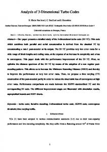
2 Equation (18) shows that the estimation of E[ wmin ] increases as the dimension D of the multiple 2 turbo code increases. Figure 5 gives the estimation of E[ wmin ] for various block lengths N and
several dimensions D, for a rate r = 1/2 turbo-code with (15,13)oct RSCC encoders (i.e. b = 2 and 2 ] is equal to 16, 38 and 60 for D = 2, 3 or 4, Pd = 4 / 7 ). For a frame size of 1000 bits, E[ wmin
respectively. Note however that, in the general case, the minimum Hamming distance of a code is generated by more complex error sequences rather than by simple weight-two input sequences.
16
2 Figure 5: Estimation of E[ wmin ] for various block lengths N with a multiple turbo-code of rate 1/2.
5. Conclusion This paper shows that the maximum spread value of a D-dimensional turbo code with tail-biting
[
]
constituent codes is upper bounded by N ( D −1) ⋅ D!
1D
. The upper bound called the sphere bound is
obtained using very simple properties of Euclidian space. It has been shown that this upper bound can be achieved in the two dimensional case, but not in the three dimensional case. For higher dimensions, the question is still open. Nevertheless, the construction of deterministic interleavers shows that the upper bound can be approached up to 92%, 88%, 91% and 80 % for D = 3, 4, 5 and 6 dimensional turbo codes, respectively. From the upper bound, it is also shown that the minimum Hamming weight of weight-two input sequences increases with the number of dimensions D for a given frame size N.
6. Acknowledgement The authors would like to thank the anonymous reviewers whose comments and suggestions have greatly helped in improving the quality of the original manuscript.
17
7. References [1] C. Berrou, A. Glavieux and P. Thitimajshima, "Near Shannon Limit Error-Correcting Coding and Decoding: Turbo Codes", Proc. ICC’93, Geneva, Switzerland, pp. 1064-1070, May 1993. [2] S. Benedetto and G. Montorsi, "Unveiling turbo-codes: some results on parallel concatenated coding schemes'', IEEE Transactions on Information Theory, vol. 42, no. 2, pp. 409-429, Mar. 1996. [3] S. Benedetto and G. Montorsi, "Design of parallel concatenated convolutional codes'', IEEE Transactions on Communications, vol. 44, no. 5, pp. 591-600, May 1996. [4] J. Hokfelt, O.Edfors and T. Maseng, "Interleaver Design for Turbo Codes Based on the Performance of Iterative Decoding", ICC '99. IEEE International Conference on Communications, Vol 1 , 1999. [5] S. Dolinar and D. Divsalar, "Weight Distributions for Turbo Codes Using Random and Nonrandom Permutations", TDA Progress Report 42-122, JPL, Aug 1995. [6] S. Crozier, "New High-Spread High-Distance Interleavers for Turbo-Codes", 20th biennial Symposium on Communications, pp. 3-7, Kingston, Canada 2000. [7] D. Gnaedig, E. Boutillon, M. Jezequel, “ Design of Three-Dimensional Multiple Slice Turbo codes”, To be published, 1st quater 2005, special issue on Turbo Processing, Eurasip Journal On applied Signal Processing. [8] E.S. Fedorov, "Elements of the study of figures" (in Russian, 1885) Zap. Mineralog. Obsc. (2) 21, 1-279. Reprinted by Izdat. Akad. Nauk SSSR, Moscow, 1953.
18