Dec 11, 2006 - xmlns:b="http://schemas.microsoft.com/BizTalk/2003" .... time performance of their algorithm becomes similar to brute-force comparison, ...... Such testing may also reveal the need for additional heuristics that we have not.
University of Waterloo, David R. Cheriton School of Computer Science, Technical Report CS-2006-47, December 2006.
MAXSM: A Multi-Heuristic Approach to XML Schema Matching Mirza Beg, Laurent Charlin, Joel So David R. Cheriton School of Computer Science University of Waterloo {mbeg, lcharlin, j2so}@cs.uwaterloo.ca December 11, 2006
Abstract Transformation of business messages from one trading partner’s definition to another, or from one business message type to another is a common requirement for enterprise data integration applications. Transforming these business messages entails resolving issues of structural and semantic heterogeneity between their schemas. In this paper, we propose an automatic schema matching approach called MAXSM, designed specifically for matching schemas in the context of enterprise data integration. MAXSM is a multi-heuristic schema matcher which employs, amongst other heuristics, a novel heuristic using WordNet for determining natural-language semantic similarity between schemas. MAXSM also introduces “transitive mappings” that can be discovered from known mappings and used to seed production of candidate mappings. We present a cogent tree spanning approach to search two schemas more effectively for node-level match candidates.
Keywords: XML Schema, Schema Matching, Schema Mapping, Semantic Matching, Tree Matching, Maximum Matching Algorithms, Location Path
1
Introduction
The adoption of XML to represent and communicate business information has increased significantly over the last decade and continues to see sustained growth. Thus, data integration scenarios in the context of electronic commerce, business-to-business integration, and enterprise application integration commonly involve the transfer and transformation of XML documents. Transformation of business messages from one trading partner’s definition to another, or from one business message type to another (within or across business processes) is a common requirement of most any enterprise data integration application. In order to transform between these business messages, corresponding schema mappings must first be defined. c 2006 Mirza Beg, Laurent Charlin, and Joel So. Permission to copy is hereby granted Copyright provided the original copyright notice is reproduced in copies made.
1
Motivated by such scenarios, we propose an automatic schema matching approach called MAXSM, designed specifically for matching schemas in the context of enterprise data integration. While our approach may be immediately useful for matching other schemas representations/definitions, we have thus far only considered and applied MAXSM to matching XML schemas. Specifically, we consider XML Schema Definition (XSD) schemas (as defined by the W3C XML Schema 1.x specification). Furthermore, by focusing on enterprise data integration scenarios, it becomes viable to maintain a repository of established schema mappings and somehow reuse that repository to enhance the accuracy of mapping candidates produced by MAXSM. The intuition here is that a repository of known mappings between schemas from the same business context/domain (e.g. schemas from the usual trading partners, used for business processes and describing products from the usual industries, etc.) will contain useful “hints” for discovering correct mappings between subsequent schemas (also belonging to that business domain). More formally stated, given two XSD schemas and a repository of established mappings (all existing in the same or related business contexts/domains), we wish to exploit the repository as well as schema semantics to automatically produce “correct” mappings between leaf/data elements or attributes defined in the two schemas. We propose MAXSM as a solution to this problem.
1.1
Contributions
MAXSM is a multi-heuristic schema matching approach. We present, amongst other heuristics, a novel heuristic which employs WordNet for determining natural-language semantic similarity between node labels. We also propose a new scheme for representing and storing known mappings in a growing repository, and describe how “transitive mappings” can be discovered from the repository and used to seed production of candidate mappings. To reduce the number of schema node comparisons made before proposing a final schema mapping, we present a cogent tree spanning approach which follows the intuition that when a very similar pair of nodes between the schemas is found, other similar pairs are likely to exist nearby (i.e. close proximity within the schema trees). We also propose a high-level pipeline architecture for implementing MAXSM.
1.2
Example Scenario
The scenario is business-to-business (B2B) electronic procurement between two frequent trading partners, whereby Company X purchases widgets from Company Y. The purchasing process involves various message exchanges: a purchase order, an invoice, a payment, and a payment acknowledgment. Let us focus on the first two messages. When Company X wishes to purchase widgets, it generates and transmits a purchase order to Company Y. Once the purchase order is received, Company Y must generate a corresponding invoice and send it to Company X. The invoice message is generated from data contained in the purchase order message. Company X designs the XSD schema for the purchase order, while Company Y designs the XSD schema for the invoice. Thus, a schema mapping between Company X’s purchase order XSD (the source schema) and Company Y’s invoice XSD (the target schema) must be created. Figure 1 shows the two schemas used in this example scenario. 2
Company X Purchase Order XSD
Company Y Invoice XSD
Figure 1: Example XSD schemas to be matched Suppose that Company X and Company Y have many business processes between them that they want to (eventually) automate. Thus, an automatic XSD schema matching tool would expedite such automation development. Furthermore, schema mappings that are defined and accepted can be stored in a repository of known mappings and used to “seed” subsequent schema mappings.
2
Related Work
Several solutions have been proposed to simplify and automate XML Schema Matching. Most are not comprehensive enough to make use of the unique structure of XML Schema and the high expressive power of the XML Schema Definition Language(XSD). The survey by Rahm and Bernstein [15] gives an overview of some of these schema matching schemes. Cilo [13] is a system that translates the source and target schemas into an internal representation and runs a Correspondence Engine and Mapping Generator to generate the mappings from source schema to target schema. Miller et al.[11] have defined an algorithm which finds derived matchings between source and target schemas given a set of substructure-level matches and match expressions using a constraint reasoning approach. Bernstein et al.[7] propose a hybrid schema matcher, Cupid, based on both structuraland element-level matching. They propose interesting heuristics using linguistic matching along with a tree scanning approach. Their algorithm separates element-level and structural similarity, then normalizes the similarity rating. In MAXSM, we embed the element-level match process into the structural matching to produce the cumulative similarity between elements.
3
XSD 1
XSD 2
Tree Encoding
Final Mapping Feedback Loop
Repository Search
REP
Max Sim Finder
Seeds
Calls
(
Tree Spanning
0.3 0.7 0.15 0.15 0.4 0.8 0.5 0.5 0.8 0.8 0.9 0.3 0.2 0.45 0.15 0.3 0.7 0.15
0.4 0.8 0.9 0.9 0.3 0.7 0.89 0.1 0.2 0.7 0.15 0.4 0.4 0.8 0.9 0.4 0.8 0.9
)
Similarity Matrix
Calls
Multi-Heuristic Similarity Calc Loc Path
DataTyp
Node Ch
Heuristic
Figure 2: An overview of MAXSM Erhard Rahm et al.[16] propose a fragment-oriented approach which focuses on matching large XML schemas. They introduce the notion of decomposing the schema into smaller fragments and reuse match results at the level of schema fragments. However, in the case where there are very small fragments of source schema matching the target schema, runtime performance of their algorithm becomes similar to brute-force comparison, making all possible node comparisons.
3
Overview of MAXSM
A high level view of the schema matching process defined by MAXSM is illustrated in Figure 2. Our goal is to generate accurate results with reasonable efficiency. We take an incremental approach to the schema matching problem. As in previous approaches [16, 7, 9], we compute the similarity of schema components by calculating the similarity function sim(n1 , n2 ) between schema elements and deduce mappings using configurable thresholds over the computed similarity values. The first phase of our algorithm scans the repository of established mappings to find potential matches between the source and the target schemas. In the second phase, the
4
algorithm traverses the schema trees starting from matches detected in phase one. This algorithm then computes similarity values between the components of the schema using the Multi-Heuristic Function on each element-pair (within proximity). Throughout this phase, similarity ratings are recorded in a similarity matrix. In the third phase, we use the computed similarity values to determine final mappings between elements of the two schemas. The resulting schema matching is presented to a human user for verification, and accepted mappings are added to the repository of known mappings.
4
MAXSM Schema Tree
XSD schemas are encoded and processed as simple tree structures within MAXSM. Our tree encoding has a tree node for every element and attribute tag defined in the XSD. All other XSD tags are excluded from the tree encoding as they have no bearing on the matching process. Furthermore, there is no distinction between element-data and attributedata – any data nodes in the XSD are simply represented by leaf nodes in the tree encoding (MAXSM is agnostic to the schema design decision of whether to represent data as XML elements or attributes). Each node in the schema tree contains all properties of the corresponding element or attribute tag defined in the XSD. These properties include the label (name), cardinality (minOccurs, maxOccurs), and data type (type). MAXSM uses this tree representation exclusively during the matching process. In fact, the final step in the matching process (discussed in section 9) actually produces final mappings in terms of the schema trees, not the XSDs. Similarly, the repository stores known mappings stated in terms of schema tree nodes and paths. Translating these mappings into mappings in terms of the original XSD schema tags is a trivial exercise; a post-processor can be written to do this translation and produce an XSLT-based map. Logically, mappings are produced between leaf nodes of the trees (since leaf nodes correspond to data elements/attributes in the XSD). A leaf node can participate in at most one mapping. That is, each leaf node can be mapped to at most one leaf node from the opposing schema tree, and mappings are bi-directional. It is also possible for a leaf node to not participate in any mapping as schema matches are not necessarily 1-1. Figure 3 shows the tree representation of our two example XSD schemas (figure 1). Leaf nodes are highlighted and dotted lines between these leaf nodes indicate the correct mappings between the example schemas. Notice that some nodes do not participate in the correct mappings. This is not uncommon (data for target nodes that are not mapped may come from auxiliary data sources/functions, post-processing, human entry, etc., and not from the source schema instance). The example schemas are used throughout the following sections to show how mappings between them are produced and proposed by MAXSM, and how the proposed mappings compare to the correct ones.
5
CompanyX_ PurchaseOrder
CompanyY_ Invoice CustomerInfo
InvoiceNumber FirstName
InvoiceDate
LastName
PONumber
ShipToAddress
PODate Street1
Buyer
Street2
Name
City
Given
Province
Surname
PostalCode
ShippingInfo
Country
PurchaseInfo
Street AptSuite
Item
City
Description
State
ItemNo
Zipcode
Qty OrderNo
Country
Price
Order Product
OrderDate ProdNum ProdDesc Quantity Amount
AmountDue ShipDate
Figure 3: Tree representation of example XSD schemas
5
Repository and Transitive Mappings
An important feature of MAXSM is its ability to reuse established schema mappings to help produce new schema mappings. The basis for this reuse is that subsequent schemas to be mapped will come from the same business domain/context as the schemas already mapped and stored in a repository, and therefore the mappings in the repository may reveal “transitive mappings” that are otherwise not necessarily apparent. A repository of known mappings essentially encodes expert knowledge about the domain. The initial generation of such a repository is an orthogonal issue. Perhaps they are grown and shared amongst trading partners, or provided by vertical standards bodies, or may simply grow from schema mappings developed manually within an organization. In any case, we assume that a repository can be readily populated by importing established schema maps, and MAXSM can function (initially) with an empty repository, albeit less efficiently. MAXSM defines a repository of known mappings as a collection of node-pairs. Each node-pair consists of two schema nodes that are known to match (from a previously accepted schema map). Node-pairs consist only of leaf-level nodes since schema mappings (in MAXSM) only map leaf nodes. The source of a node (i.e., which schema it came from) is not retained in the repository. This is by design. The repository represents known schema node mappings as discrete node-pairs, it is not concerned with overall schema maps. This makes the individual known node mappings schema-agnostic and thus more versatile when being compared to nodes in to-be-matched schemas. To represent a node in our repository, we use a location path expression that is based loosely on XPath 1.0 Location Paths [19]. A location path of a node is the nested path to that node within the schema tree, starting from the root. Thus, our repository contains pairs of schema-agnostic location paths representing pairs of schema nodes that are known to be mapped from some established schema mapping. We define a location path expression as follows (this is similar to XPath Location Path 6
expressions, but customized in terms of verbosity and readability for our purposes): [root node]/../[inner node] ∗ /../[leaf node] where each root node, inner node, leaf node contains name =?, minOccurs =?, maxOccurs =?, type =? Using our repository to discover potential schema mappings is intuitive. Given two schemas to be matched, we query the repository for node-pairs where one side of the pair is similar to a node in the first schema tree, and the other or same side of the pair is similar to a node in the second schema. When such a pair can be found in the repository, we can conclude that there is some level of similarity or association between the said nodes in the two to-be-matched schemas. For example, suppose we wanted to find a mapping for two schemas, Schema1 and Schema2. Suppose Schema1 contains a node A, and Schema2 contains a node B. Now suppose that the repository contains a known mapping: node-pair (X,Y) from some established schema mapping. If we compare the nodes in Schema1 with the nodes in the repository and find that A is similar to X, then subsequently compare the nodes in Schema2 with X and Y and find that either X or Y is similar to B, then it must be that A is also similar to B. That is, if A is similar to X, X is known to be mapped to Y, and X or Y is similar to B, then we can conclude that A is also similar to B. In essence, we are using the repository to determine transitive similarities between nodes. The fact that both already-mapped and to-be-mapped schemas come from the same business domain/context is key. This means, for example, that schemas come from the usual trading partners and are created by the usual schema designers, that they are used for business processes and to describe products belonging to the usual industries, etc. As such, the schemas may be more homogeneous in design (e.g., using common acronyms, jargon, or structure) and this increases the likelihood that nodes in known mappings will have similarities with nodes in to-be-mapped schemas. Section 7 discusses how the repository is searched to find preliminary mappings.
6
Multi-Heuristic Similarity Function
To evaluate the similarity between leaf nodes, we use an aggregation of multiple heuristics. The idea is to have a similarity function that takes two nodes (n1, n2) as input and outputs a score (sim(n1 , n2 ) ∈ [0, 1], with 1 being perfect similarity) based on the aggregation of similarity heuristics. The three heuristics that are core to MAXSM consider all information expressed in XSD schema: name of the nodes, their paths, type, and cardinality, and the structure of the schema tree. The name and path of a leaf node are particularly important and require both syntactic and semantic analysis during comparison. Our similarity function represents a simple and efficient way of combining different heuristics that each exploit key features of XSD schemas. Moreover, this approach allows 7
position 3
position 2
position 1
position 0
CompanyX_ PurchaseOrder
Customer Info
ShipTo Address
Province
0.7
0.6
0.8
0.7
CompanyY_ Invoice
Buyer
Shipping Info
State
Figure 4: Example of token comparisons made by location patch matching heuristic. for addition (or removal) of heuristics (see section 6.4). The following sections discuss each core heuristic in detail.
6.1
Location Path Matching
Every node in a schema tree has a unique location path in the form described in section 5. A location path encodes information about the node that it is referencing, information about each of the nodes from root to the node being referenced, and the relative position of these nodes within the path. Thus, when comparing two schema nodes based on similarities in their location paths, similarities in the ancestors of the nodes being compared are implicitly considered as well. The location path matching heuristic defines a similarity function simLP (n1 , n2 ) ∈ [0, 1] which compares the location paths of node n1 and n2 to produce a similarity value. The location paths are compared in terms of string pattern and natural-language semantic similarities of “tokens” in the location paths, as well as the relative ordering of these tokens within the paths. A token represents the information enclosed in square brackets in a location path (i.e., each term or entry seperated by “/”s). To determine the string pattern similarity of two node names, the similarity sub-function discussed in section 6.1.1 is called. To determine the natural-language semantic similarity, the sub-function discussed in section 6.1.2 is called. In this section, let simwords (w1 , w2 ) be the equally-weighted average of similarity ratings from these two sub-functions. Thus, simwords (w1 , w2 ) gives a similarity rating for words w1 and w2 based on their string pattern and linguistic semantic similarities. The location path matching heuristic simLP (n1 , n2 ) produces a similarity value by comparing the location paths of n1 and n2 , n1 .locationPath and n2 .locationPath respectively. More specifically, this heuristic compares the name property of the tokens in the location paths using simwords (w1 , w2 ). Each token in a location path is assigned an ordinal position value, beginning with the right-most tokens. Using our example schemas, consider the location paths for the Province node in Company X’s purchase order schema, and for the State node in Company Y’s invoice schema. Figure 4 illustrates how tokens in these location paths are assigned ordinal position values. Tokens at position 0 are of greatest importance since they represent the node that the location path references. Tokens with increasingly higher position values have relatively less importance as they represent nodes that are further away (ancestrally) from the node referenced by the location path. 8
The location path matching heuristic determines simwords (w1 , w2 ) for pairs of tokens that are in the same ordinal position. Intuitively, comparisons are not made between pairs in different ordinal positions as that comparison is meaningless (in the context of location path matching). For example, there is no reason to compare a token at position 0 that represents a leaf node in one schema, with a token at position 3 that represents an inner node in another schema. It is intuitive to only compare tokens in the same ordinal position. Thus, simwords (w1 , w2 ) is calculated for each pair of like-position tokens, as shown for the example location paths in figure 4. In the case where n1 .locationPath and n2 .locationPath comprise different numbers of tokens, the location path with the greater number of tokens will have the leftmost tokens ignored and not included in any comparison. This follows the intuition that only like-position tokens should be compared. If one location path has a greater number of tokens than another, it means that the node being referenced by the longer location path is deeper in its schema tree than the node being referenced by the shorter location path, in its schema tree. Thus, it is meaningful to compare only up to the height of the shorter path (which includes up to the root of that schema tree). Figure 4 illustrates the tokenization, position assignment, and comparison of Province.locationPath and State.locationPath. The dotted lines indicate the value-pairs passed to simwords (w1 , w2 ) and the similarity rating returned. Recall that simwords (w1 , w2 ) is based on string pattern similarities as well as natural-language semantic similarities. This explains why simwords (“ShipToAddress”, “ShippingInfo”) is relatively high, and why simwords (“CustomerInfo”, “Buyer”) is relatively low (in the first case, there is substantial string pattern and semantic similarity, while in the second case, there is very little string pattern similarity). To derive a final value for simLP (n1 , n2 ), a weighted average of the calculated simwords (w1 , w2 ) values is taken. Intuitively, we want the rightmost similarity values to carry the most weight, with decreasing weights moving leftwards. The basis for this is that we care most about the similarity rating of the tokens representing the nodes being referenced by the location paths, and care increasingly less about the similarities of tokens representing nodes that are further away (ancestrally) from the nodes referenced by the location path. Thus, we assign weights 1 defined as 2(1+p) where p is the ordinal position of the tokens being compared. In order to have the weights sum to 1, we assign the leftmost weight as always being 21p , i.e., the leftmost value will carry the same weight as the second-to-leftmost value. This is a mere simplification. So for our example, simLP (Province, State) is calculated as: 1 2 (0.7)
+ 14 (0.8) + 81 (0.6) + 18 (0.7) = 0.7125
This scheme ensures that the relative ordering of the tokens are considered in the overall similarity rating produced by this heuristic. That is, highly similar token pairs that are relatively out-of-order are not considered and cannot cause the overall similarity value produced to be invalidly high. The following sub-sections detail the sub-functions called by the location path matching heuristic. 6.1.1
String Pattern Similarity Function
This function deals with string pattern similarity and matches nodes with respect to character use and formatting in their names. More specifically, this function maps a pair of 9
strings w1 and w2 to a similarity rating between 0 and 1: sim(w1 , w2 ) ∈ [0, 1] – the larger the value returned, the greater the similarity between w1 and w2 . In our context, w1 and w2 are the names/labels of two schema nodes being compared. The problem of assigning distance or similarity values to a pair of strings/words based on pattern matching (versus natural-language semantic matching) is a well-studied one in the database community, as well as in AI and statistics [3]. A common metric used for quantifying string pattern similarity between two strings w1 and w2 is the edit distance between them. In general, edit distance is defined as the total cost or number of operations required to convert w1 to w2 . Typical edit operations are character insertion, deletion, replacement. Depending on application and context, different costs may be assigned to each operation. Edit distances are most often normalized to a value in [0,1]. Cohen et al. [3] carried out an empirical comparison of various string distance/similarity functions. They ranked these functions in terms of “accuracy” for use in an automatic string matching scheme, in which pairs of matching strings are proposed based on similarity/distance ratings produced by each function. Similar to evaluating schema matching schemes, “accuracy” describes how close a proposed set of pairs/matchings is to an intended set (as intended by a human matcher). Since this experiment design closely models how a string distance function is used in MAXSM, the findings reported are directly relevant for our XML schema matching approach. We adopt the Monge and Elkan [12] string pattern similarity function sim(w1 , w2 ). Monge and Elkan define a recursive matching scheme for comparing two strings w1 , w2 . In their scheme, w1 and w2 are decomposed into substrings w1 = s1 . . . sk and w2 = t1 . . . tl , then substrings are recursively compared using some secondary distance function sim0 (s, t) [12]. The Monge and Elkan string pattern similarity function performed most accurately among the several edit-distance-based similarity functions compared in [3]. 6.1.2
Semantic Similarity Function using Wordnet
This function deals with semantic similarity and matches nodes with respect to the meanings of their names. The motivation for using this comes mainly from the field of natural language processing and some of their methods [2]. Successful methods such as the one from Jiang [6] rely on WordNet, a lexical taxonomy http://wordnet.princeton.edu/. Furthermore, the semantic understanding of node names seems like a necessary tool due to the complexity of schema matching. To find similarities between two concepts (a particular definition of a certain word), these methods usually use the hyponymy relations given in WordNet. Hyponomy relations are “IS-A” relations. For example, a “car” is a “motor vehicle” which in turn is a “self-propelled vehicle”. All the words in WordNet are therefore in a tree-like hyponomy structure. Intuitively, given two leaf nodes from the XSD schemas, their position relative to each other in this tree that will determine their degree of similarity. Unlike [7], we only use hyponomy relations as the results of Budanistsky [2] find that this is sufficient. Jiang’s method uses the following two ideas to evaluate semantic similarity. First, the closer two words are in the hyponomy structure, the closer their meanings are. This is referred to as the Edge-Based Approach and was first proposed by Rada [14]. The simple ideas is to count the number of edges in the hyponomy tree and use this distance as the measure of the similarity of two words. As explained in [6], higher density areas in the
10
tree make for closer semantic similarity. Also, the lower in the hierarchy a concept is, the closer its meaning is to its neighbors (thus the higher the weights of the edges should be). Each child of a parent could also have a different importance. This could be based on a previously seen corpus, for example. The second idea is to look at how much information in common the two concepts give. This is called Information Content (IC). It is based on information theory and was first proposed by Resnik [17, 18]. Technically, you can calculate this value by looking at the frequency of some concept which subsumes both concepts. In information theory, a term which is more frequent is considered to give less information (IC = log−1 (P (c)) where P (c) is the probability of a term). In our case, higher terms subsume lower ones (so that the IC of the root of the tree is 0). Of course, when we talk about frequencies of words, we need to learn those frequencies from some corpus. In addition, the corpus could be tagged with WordNet to get the correct concept for each word. As Jiang did, we use the SemCor corpus [10] - this will also make us use a Good-Turing estimation with linear interpolation for the probability estimations. In their paper, Jiang proposes two formulas, one being a simplified version of the other (floating parameters have been set). Furthermore, Jiang shows that fixing the tuning parameters does not result in significant changes. Thus, we use the simplified equation, as follows: Dist(w1 , w2 ) = IC(c1 ) + IC(c2 ) −2 × IC(LSuper(c1 , c2 )) Where w1 , w2 are the words we are trying to match, ci the concepts related to these word and LSuper is the lowest common parent that c1 and c2 have. Of course, for inclusion into our aggregation function we need to normalize the Dist value. One way is to set a minimum threshold on the probability value (if the probability is under that value we raise it to the threshold). For example, if this threshold is 0.001 than the Dist will have a maximum value of 6.0 (Dist = 3 + 3 − 2 × 0). After we have normalized it, we simply take its complement (1 − Dist) to get a similarity value. Finally, to get the sense of a word (ci = sem(wi )), we use its most common sense as given by WordNet.
6.2
Data Type and Cardinality Matching
Matching schema nodes based on data type and cardinality is a common and reliable similarity measure. Both data type comparison and cardinality comparison are considerably more deterministic than, say, linguistic semantic matching. For our purposes, we define a similarity function using data type and cardinality comparison as: Given a node pair (n1 , n2 ) where n1 ∈ S1 and n2 ∈ S2 and S1 and S2 are two schemas being matched we define, simDT +Car (n1 , n2 ) = δ ∗ simdatatype (n1 , n2 ) +∆typeSim ∗ (1 − δ) ∗ simcardinality (n1 , n2 )
Note that simDT +Car (n1 , n2 ) ∈ [0, 1]. δ and 1 − δ are the proportional weights given to the similarity of the data type and the cardinality of the element. We only give a weight 11
to the cardinality of elements if their data types match. This is captured by the ∆typeSim parameter which corresponds to a binary value in {0,1} based upon data type similarity. XML schema specification [20] allows for many different data types and regular expressions which makes this heuristic more significant compared to data type matching in relational databases. For example, on top of the usual integer, float, double, string etc. data types, XML Schema accepts extensions to data types (e.g. year field can be declared as an value in [1900-2050]). Also, many string data types can be represented as regular expressions. For example, a field representing telephone numbers is usually an integer, but is represented as strings allowing for special characters such as ‘-’ and ‘x’ etc. Since XML Schema allows for the definition of very specific data types, data types matches are reasonable indicators of candidate mappings. This heuristic also has to deal with “equivalences” between data types. For example, a float and an integer can in some cases be used interchangeably, while a float and a string typically cannot. We base this idea and use the actual sets of related types from [5]. The other part of the equation is matching the cardinality of an element in the schema (simCar or equivalently simcardinality ). Elements in a schema may occur with a varying degree of cardinality. The cardinality of an element expresses the ability of that element to be repeated in an instance of that schema. Matching the cardinality of an element gives an idea of the semantic ‘closeness’ of elements of the two schemas which we use in this heuristic. In XML, the cardinality of elements can be found through minOccurs, maxOccurs attributes. The weighted cardinality between two nodes is represented in the similarity function as (1 − δ) ∗ simcardinality (n1 , n2 ). Here is a simple function to calculate this similarity (in which we can flip the denominator so that it is always ∈ [0, 1]): � � maxOccursn1 − maxOccursn2 abs minOccursn1 − minOccursn2 The example scenario in Figure 5 illustrates how MAXSM’s multi-heuristic module will compute similarity based upon data type and cardinality values. If we compute similarity value simdatatype (P rice, n2 ) for P rice in S1 and n2 in S2 respectively, then we would get the maximum similarity value for simdatatype (P rice, Amount) where the closest data type to double is f loat. They would give an exact match for cardinality. An interesting scenario for cardinality matching would be for the complex-type Item. In the case of Item, it would give a max value for simcardinality (Item, P roduct) where it is not possible to actually compare the complex types and we assign ∆typeSim a 1 so that the similarity function can be computed for the cardinality of the element.
6.3
Node Characteristics Matching
This heuristic compares the elements of two schemas based upon their position in the schema tree and the structure that extends from them. It tries to detect similar subtrees between two XML schemas by comparing node characteristics: number of children, height from the leaf node, number of siblings, and depth. To define the similarity function for this heuristic, we compute the structural similarity between two given nodes n1 and n2 in schema S1 and schema S2 , respectively, by the
12
Order
PurchaseInfo
simCar(Item, Product) > simCar (Item,Name ) &
Cardinality Match
Cardinality: unbounded
Item
Description
ItemNo
Type: string
Cardinality: 100
Product
ProdNum
Type: string
Qty
Price
Type: integer
Quantity
Type: string
Type: long
Amount
ProdDesc
Type: double
Type: float
Type: string
Datatype Match simDT(Price, Amount) > simDT (Price, ProdNum) & simDT (Price, ProdDesc) & simDT (Price,
Figure 5: An illustration of Data type and Cardinality matching Eventual Node Characteristics Match
# Children: 3, # Siblings: 5, Height: 2
# Children: 3, # Siblings: 1, Height: 2
Order
PurchaseInfo
simNodeChar(Item, Product) > simNodeChar (Item,Name ) # Children: 4, # Siblings: 2
OrderNo
Item
ItemNo Qty
ShipDate
Product
OrderDate Description
AmountDue
Node Characteristics#Children: 4, # Siblings: 2 Match
ProdNum
Quantity
Price ProdDesc
Amount
Figure 6: An illustration of Node Characteristics matching equation simN C (n1 , n2 ) = λ ∗ simnodeSimilarity (n1 , n2 ) X +(1 − λ) ∗ simsubT reeN odes (n1,i , n2,j )
where simN C (n1 , n2 ) ∈ [0, 1]. The first part of the equation uses the actual similarity between the two nodes n1 and n2 .That is, for each characteristic it calculates the difference between the two nodes. The second part of the formula does the same for every child of the current nodes (n1,i or n2,j respectively) and averages them out. The idea is to find matching structures. In any case, the parameter λ can be tuned according to scenario and context. The interesting point to note here is that subtree structure matching still has value even though the two nodes may differ drastically in their characteristics. Figure 6 illustrates this heuristic. If we compute the similarity function presented in this section on Item, we would get a maximum similarity value for simN C (Item, n2 ) with n2 13
being P roduct. This is because Item has not only the same number of children but also the same number of siblings. In addition, the height from the bottom of the tree for the nodes Item and P roduct is the same. The second component of the structural similarity function would also yield a high value for simsubT reeSim (Item, P roduct) because of the previous matchings which would have found the subtrees very similar. This similarity value would eventually help determine the similarity of the parent nodes P urchaseInf o and Order.
6.4
Combining Heuristics
In this section, we discuss how to combine our heuristics to give a final similarity value to a pair of nodes. The idea is to do a weighted average of the heuristics. The weights are given a default value but are tunable according to specific context/scenario. The equation for this summation is given by simM ulti−Heuristic (n1 , n2 ) = α1 ∗ simLP (n1 , n2 ) +α2 ∗ simDT +Car (n1 , n2 ) + α3 ∗ simN C (n1 , n2 ) where simLP is the similarity calculated by Location Path matching, simDT +Car is the similarity computed by the Data type and Cardinality matching, simN C is the similarity from Node Characteristics matching. To make sure that the P range of the function is correct (∈ [0, 1]), we require that the following condition is met i αi = 1 Concerning the default values, we will give a higher score to the first heuristic. This is because it contains two different functions which are both very meaningful. By default, we set α1 to be α2 + α3 . For simplicity, we refer to the above function as sim(n1 , n2 ) throughout this paper.
7
Matching Step I: Preliminary Mappings
The first step of MAXSM is to produce preliminary mappings by searching for “transitive mappings” in the repository. Preliminary mappings are based solely on similarities between nodes in the repository and nodes in the schemas being matched. Similarities between nodes in the schemas themselves are not considered at this stage. Preliminary mappings are used in the second step of MAXSM (section 8) as “seeds” or hints of good mapping candidates and also serve as starting points for a tree-spanning search for additional candidates. We are given two schema trees S1 and S2 to be matched, a repository R of node-pairs (each pair representing an individual known mapping), and the multi-heuristic similarity function simM ulti−Heuristic (n1 , n2 ) (let us henceforth use sim(n1 , n2 ) for short). Let τ1 ∈ [0, 1] be a user-configurable threshold for “acceptable” similarity ratings. To find preliminary mappings between S1 and S2 , the following three sub-procedures are performed: Search 1: For each leaf node n1 in S1 , find all node-pairs p = (x, y) in R where max(sim(n1 , x), sim(n1 , y)) ≥ τ1 . Store all such n1 , p, and simSearch 1 , where simSearch 1 = max(sim(n1 , x), sim(n1 , y)). Thus, Search 1 finds all repository node-pairs that contain nodes that are sufficiently similar to leaf nodes in the first schema.
14
Search 2: For each (n1 , p = (x, y), simSearch 1 ) 3-tuple stored during Search 1, find all leaf nodes n2 in S2 where max(sim(n2 , x), sim(n2 , y)) ≥ τ1 . Store all such n1 , p, simSearch 1 , n2 , and simSearch 2 , where simSearch 2 = max(sim(n2 , x), sim(n2 , y)). Thus, Search 2 finds all leaf nodes in the second schema that are sufficiently similar to nodes in node-pairs found by Search 1. We now have a collection of (n1 , p, simSearch 1 , n2 , simSearch 2 ) 5-tuples returned by Search 2 (the results of Search 1 can now be discarded). Each tuple represents a transitive mapping: leaf node n1 in S1 is similar to node x and/or y in node-pair p, node-pair p comes from the repository of known mappings and therefore x maps to y, and x and/or y is similar to leaf node n2 in S1 . Therefore, n1 can be transitively mapped to n2 . However, the collection may contain “collisions”. That is, a leaf node in S1 or S2 may be included in more than transitive mapping. This cannot remain as leaf nodes can participate in at most one mapping. Thus, we must resolve the collisions by discarding transitive mappings that include leaf nodes already included by another transitive mapping. To decide which transitive mapping to keep when faced with collisions, we consider which mapping has the greatest transitive similarity. Resolve Collisions: For each (n1 , p, simSearch 1 , n2 , simSearch 2 ) 5-tuple returned by Search 2, calculate the transitive similarity simTrans = (simSearch 1 + simSearch 2 )/2 and store the 3-tuple (n1 , n2 , simTrans ). The corresponding 5-tuple can be discarded. This gives us a collection of simplified transitive mappings between leaf nodes in the two schemas, with a (transitive) similarity rating for each. Now sort the 3-tuples in the collection by decreasing simTrans . Let P be a set of node-pairs, each node-pair representing a preliminary mapping derived from the repository of known mappings. P begins as an empty set. Then, for each (n1 , n2 , simTrans ) in the sorted collection (beginning with the tuple with the greatest simTrans ), add node-pair (n1 , n2 ) to P if-and-only-if (n1 ∈ / P ∧ n2 ∈ / P ). What we achieve is a set of preliminary mappings (a leaf node in S1 mapped to a leaf node in S2 ) such that each mapping/node-pair (n1 , n2 ) has the greatest (transitive) similarity rating of all possible leaf node-pairs containing n1 or n2 . By definition, node n1 and n2 cannot appear in any other node-pair in the set. Said another way, the set of preliminary mappings consists of the most transitively similar pairs of leaf nodes (one from each schema), with each node participating in exactly one pair.
8
Matching Step II: The Similarity Matrix
In this step, the schema trees are traversed and a similarity matrix is populated with calculated similarity ratings. The problem is two fold: first, find a matching in the trees which corresponds to our constraints, second, maximize (span) that matching. The first step is to calculate the similarity functions (sim(n1 , n2 )) between the nodes of the two trees. If possible, we can simply do a (brute-force) pairwise comparison of leaf nodes in one tree to each leaf node in the other tree. Values returned by this procedure which are above the user defined threshold are added to a similarity matrix. Since we believe that this brute-force approach might not be feasible for larger schema, we propose an approximation which takes advantage of specific characteristics of our problem. First, let us define the similarity matrix. This matrix is simply a N1 ×N2 storage (where 15
Buyer
Name
Given
Surname
CutomerInfo
ShippingInfo
State
City
ShipTo
FirstName
City
Province
LastName
Figure 7: This shows the Tree Spanning procedure on a subset of the XSD schemas previously discussed N1 and N2 are respectively the number of leafs in trees n1 and n2 ) containing, for each cell, the value of the similarity of the two nodes (or zero if this value is unknown). We refer to the similarity matrix as being “full” when it is fully populated. We now propose a more efficient node-comparison scheme which relies on matches given by Step I. The idea is to use these matches, as seeds or starting points, to make an educated spanning search into our two trees. Intuitively, we want to start at the seeds and compare surrounding nodes. We then span-out like this until a maximum number of nodes have been matched. The idea is that if two nodes match, their neighbors have a higher chance of matching as well. The heuristic goes as follows (algorithm 1). For each match given by Step I, we check the two nodes in the trees with the similarity function. If the value of the function is higher than the threshold (τ1 ), we consider this seed to be a definitive match. Let us also note that since such a match comes from the repository, we add a bonus value to the similarity function (this value is configurable). We then “grow” from these seeds to find other matches. That is, we try to match the siblings and parents of these matched nodes. Of course, if the similarity function did not return a score above the threshold, we discard the seed. For each “acceptable” seed, we try to match parents, then grandparents, and then recurse on their children in this way until we cannot find matches in two subsequent layers. If matches have not been found within two levels from a seed, then the seed has reached its “helping capacity”. Intuitively, two levels away is a good trade-off between efficiency and accuracy. We also have a second threshold τ2 which is used when we are not comparing leafs. Notice that, since we only want to match leaf nodes with leaf nodes, we do not cross-compare internal nodes and leafs. In Procedure 1, c(n) refers to the set children of a node n, s(n) to the set of all siblings of a certain node, and p(n) to the parent of a node (which is unique). This is an approximation technique which may significantly reduce the time to match the nodes (it’s lower bounded by N ). To illustrate an example of this procedure, we take a subset of the original XSD schema shown in figure 8. We start with the seed “City” which was given by Step I. The procedure then compares the seed-pair again to make sure they are actually matched. It then calls the GoUpfunction which would in turn call the similarity function on all the pairs of siblings of “City”. If there is a match, e.g. between State and Province, then we call GoDownwith the parents (“ShippingInfo” and “ShipTo” respectively). We then compare the siblings of these parents. The obvious fact is that the siblings of “ShipTo” are leafs. So we would actually go down and compare these leafs with the children of the siblings of “Name” (in this case
16
“ShppingInfo”). Once these comparisons are done, we go up (at least one more level) and compare “Buyer” with “CustomerInfo”. Whether or not we go up again is based on the results of these matches and the ones of the siblings of “ShippingInfo” and “ShipTo” (this refers to the rule about visiting a maximum of 2 levels higher from a seed-match). Procedure 1 Tree matching 1: for all seeds, si,n , do 2: n1 = si,1 , n2 = si,2 3: if sim(n1 , n2 ) + bonus > τ1 then 4: Store this value in the full similarity matrix 5: end if 6: GoUp(n1 , n2 ) 7: end for 8: 9: 10: 11: 12: 13: 14: 15:
Func GoDown(n1 , n2 ) for all pairs of siblings, s(n1 ) × s(n2 ) do if sim(n1,i , n2,i ) > τ1 then {or τ2 if the nodes are not leafs} Update the values in the full similarity matrix GoDown(c(n1,i ), c(n2,i )) {unless they are leaf nodes} end if end for
16: 17: 18: 19: 20: 21: 22: 23: 24: 25: 26:
9
Func GoUp(n1 , n2 ) for all pairs of siblings, s(n1 ) × s(n2 ) do if sim(n1,i , n2,i ) > τ2 then Update the values in the full similarity matrix GoDown(p(n1,i ), p(n2,i )) end if end for if none have matched then GoUp(p(n1 ), p(n2 )) {unless they are root nodes} end if
Matching Step III: Final Mappings
In this step, we generate a final set of proposed mappings based on results captured in the similarity matrix, while attempting to maximize the total number of proposed mappings (i.e., the map coverage). We start with the similarity matrix built in the previous step and now need to find the maximum edges. Note that this is not necessarily the maximum number of matchings. Furthermore, each node can only participate in one match. Thus, this process is not straightforward as the same leaf node may have the same match value for different leafs in the other tree. Formally, for each leaf node in one tree, n1 we could express our objective function as f (n2 ) = arg maxn1 sim(n1 , n2 ) An intuitive way to solve the problem is to always take the match that has the maximum 17
n 1,1 n1,2 n 1,3
n 1,1 n1,2 n 1,3
n 1,1 n1,2 n 1,3
n 2,1 0.9
0.7
0.3
n 2,1 0.9
0.7
0.3
n 2,1 0.9
0.7
0.3
n 2,2 0.6
0.8
0.5
n 2,2 0.6
0.8
0.5
n 2,2 0.6
0.8
0.5
n 2,3
0.8
0
n 2,3
0.8
0
n 2,3
0.8
0
0
0
0
Figure 8: Given the similarity matrix this shows the process which leads to finding the maximal matchings value in the matrix. Once this has been taken, we cross out (or zero-out) the column and row of the two chosen nodes. We do this until all the nodes have been matched or the maximum value left is under the threshold. The complication comes when the maximum is not unique on its row or column. To deal with these, we simply check the next largest value. The one that gives us this second maximum value is the one we accept. Formally, this has a complexity of O(N 2 log N + (N 2 )). The first term is to sort the matrix and the second to find maximum matchings. The second term is somewhat loose but it is still upper-bounded by the first. An example of this algorithm is given in figure 8. We are given a similarity matrix (shown at the left in the figure). Then (middle matrix), we find the maximum value (0.9) and call n2,1 and n1,1 a match. We also cross their respective rows to indicate that these nodes have been matched. In the next step, we find a conflict: there are two maxima (0.8) in the same column. The algorithm tries both. Since it is better to have a third match of 0.5 than 0, we end up matching n2,3 and n1,2 which leaves the match of n2,2 with n1,3 . Interestingly this problem has the same feel as the bipartite weighted matching problem. The main difference is in the objective function. In one we are trying to maximize the total number of matchings, in the other, as in our problem, we want the maximum matching for√each node. In any case, the best technique [1] to solve the assignment problem runs in O( N1 m log(N C)) (this is using the Cost Scaling algorithm). In our case, the number of arcs m ≤ N1 N2 .
10
Experiments Design
Intuitively, for matching XML schemas, our tree spanning algorithm should be faster than the brute force approach (which makes all possible node comparisons). Our intuition is that given an appropriately sized repository, it should also perform better in terms of accuracy (F-measure) than the brute force approach. We need to compare these two approaches using differently sized schemas. We expect that matching larger the schemas will benefit most from using the tree spanning approach. The experimentation here is typical of any schema matching approach. There are also various aspects unique to MAXSM that we must verify. Firstly, we need to quantify the efficacy of the repository of known mappings. We would like to see how the size of the repository might affect the accuracy of our matchings. So, we’d like to run experiments with different repository sizes. Of course, another consideration is the homogeneity between established schema mappings that are imported into the 18
repository, and subsequent to-be-matched schemas. To control the second variable during experimentation, we select a single business domain (and schema sources) from which to match schemas. For example, we could take schemas from the financial services vertical, and ones that belong to the same electronic banking standards body. This ensures that all test schemas exist in the same business context. We would then run MAXSM against, say 20 pairs of schemas to be matched (with an empty repository), then run MAXSM against another 20 pairs of schemas to be matched (this time with the repository populated by the previous 20 schema maps), then run it again with another 20 pairs of schemas (this time with known mappings from the cumulated 40 schema maps), etc. Secondly, we need to gain better understanding of the effects of the user-configurable thresholds in MAXSM when faced with real-world schemas to be matched. We have left the burden of setting the various thresholds and similarity weights to the user. Although this is a reasonable approach since only users have domain-specific knowledge of the characteristics of the schemas in their domain/context, we would still like to give reasonable default values to all of these configurable parameters – we must first learn what “reasonable default values” are based on experimental results. We would also like to understand empirically how sensitive match accuracy in MAXSM is to changes to the various threshold values. To learn these things, we must conduct experiments using various value ranges for the configurable thresholds. Such testing may also reveal the need for additional heuristics that we have not yet considered, or the depreciation of heuristics that we have. Finally, we need to compare MAXSM against other available XML schema matchers. A good measurement will then be to compare MAXSM’s match accuracy with that of other approaches, when matching the same pairs of schemas. Since we have built on the ideas of some existing approaches and ideas (as referenced throughout the paper), we expect MAXSM to outperform, but of course must verify this experimentally.
11
Conclusions
We have proposed a comprehensive approach called MAXSM for matching XML schemas. MAXSM is a multiple-heuristics based matcher that incorporates some novel features such as the repository of known mappings, a natural-language matching function that uses WordNet, and a tree spanning technique for discovering clusters of similar nodes. We also present a location path structure to reference nodes in a schema tree, and corresponding matching heuristic that determines node similarities based on their location paths. Furthermore, we present matching heuristics which consider data type, cardinality, and node-tree characteristics similarities. MAXSM has been designed from the ground-up as a matching scheme exclusively for XML schemas in the enterprise data integration space. While MAXSM has not yet been implemented, we expect positive results due to the deliberateness of its design to address XML schema matching in a focused context.
12
Future Work
An idea from [7] was to use true machine learning for the schema matching problem. Some groups [8] have already done so. We could also benefit from these in at least two different
19
aspects. First, like [8] instead of leaving the choice of the similarity weights to the user we could learn them. An algorithm such as the Winnow could be used to do so. An alternative idea to our tree spanning would be to pre-order the leaf nodes of one tree according to each heuristic. We would basically have ranked lists and could then use a combine rank algorithm (such as the Threshold Algorithm [4]) to find the top node given another a leaf from the other tree. Thus, the leaf nodes in one tree would be ranked and the nodes in the other would act as queries. The problem of course is to pre-order the leafs in one tree without knowing about the leafs in the other. One solution would be to sort them using basic metrics needed in the heuristics. The problem of course then becomes finding those metrics for each heuristic. Finally, in addition to actually implementing and testing MAXSM as presented, we also want to consider making MAXSM a more general solution, testing it both conceptually and experimentally for use with other schema representations, beyond XSD. The ideas and approaches used in MAXSM are not fundamentally coupled to XSD and the general feeling is that it can be applied to any schema representation that can be encoded in our schema tree structure. Even the efficacy of the repository and reuse of mappings is independent of schema representation – it is more dependent on the schema matching context or domain, and the homogeneity of schemas in that domain.
About the Authors Mirza Beg is a Masters candidate at the University of Waterloo, School of Computer Science, working in the Networks and Distributed Systems Group. Laurent Charlin is a MMath candidate at the University of Waterloo, School of Computer Science, working in the Artificial Intelligence Group. Joel So is a Master’s candidate at the University of Waterloo’s School of Computer Science, working in the Workflow Research Group in Healthcare Informatics.
References [1] R. K. Ahuja, T. L. Magnanti, and J. B. Orlin. Network flows: theory, algorithms, and applications. Prentice-Hall, Inc., Upper Saddle River, NJ, USA, 1993. [2] A. Budanitsky. Semantic distance in wordnet: An experimental, application-oriented evaluation of five measures. In Second meeting of the North American Chapter of the Association for Computational Linguistics (NAACL-2001), pages 29–34, Pittsburgh, PA, June 2001. [3] W. W. Cohen, P. Ravikumar, and S. E. Fienberg. A comparison of string distance metrics for name-matching tasks. In IIWeb, pages 73–78, 2003. [4] R. Fagin, A. Lotem, and M. Naor. Optimal aggregation algorithms for middleware. In PODS ’01: Proceedings of the twentieth ACM SIGMOD-SIGACT-SIGART symposium on Principles of database systems, pages 102–113, New York, NY, USA, 2001. ACM Press. [5] B. He, K. C.-C. Chang, and J. Han. Discovering complex matchings across web query interfaces: a correlation mining approach. In KDD ’04: Proceedings of the tenth ACM SIGKDD international conference on Knowledge discovery and data mining, pages 148–157, New York, NY, USA, 2004. ACM Press.
20
[6] J. J. Jiang and D. W. Conrath. Semantic similarity based on corpus statistics and lexical taxonomy. CoRR, cmp-lg/9709008, 1997. [7] J. Madhavan, P. Bernstein, and E. Rahm. Generic schema matching with Cupid. In Proc. 27th VLDB Conference, pages 49–58, 2001. [8] R. McCann, B. AlShebli, Q. Le, H. Nguyen, L. Vu, and A. Doan. Mapping maintenance for data integration systems. In VLDB ’05: Proceedings of the 31st international conference on Very large data bases, pages 1018–1029, Trondheim, Norway, 2005. VLDB Endowment. [9] S. Melnik, H. Garcia-Molina, and E. Rahm. Similarity flooding: A versatile graph matching algorithm and its application to schema matching. In ICDE ’02: Proceedings of the 18th International Conference on Data Engineering (ICDE’02), page 117, Washington, DC, USA, 2002. IEEE Computer Society. [10] G. A. Miller, C. Leacock, R. Tengi, and R. T. Bunker. A semantic concordance. In HLT ’93: Proceedings of the workshop on Human Language Technology, pages 303–308, Princeton, New Jersey, USA, 1993. Association for Computational Linguistics. [11] R. J. Miller, L. M. Haas, and M. A. Hern´andez. Schema mapping as query discovery. In A. E. Abbadi, M. L. Brodie, S. Chakravarthy, U. Dayal, N. Kamel, G. Schlageter, and K.-Y. Whang, editors, VLDB 2000, Proceedings of 26th International Conference on Very Large Data Bases, September 10-14, 2000, Cairo, Egypt, pages 77–88. Morgan Kaufmann, 2000. [12] A. E. Monge and C. Elkan. The field matching problem: Algorithms and applications. In Knowledge Discovery and Data Mining, pages 267–270, 1996. [13] L. Popa, Y. Velegrakis, R. J. Miller, M. A. Hern´andez, and R. Fagin. Translating web data. In VLDB, pages 598–609, 2002. [14] R. Rada, H. Mili, E. Bicknell, and M. Bletner. Development and application of a metric on semantic nets. IEEE Transactions on Systems, Man, and Cybernetics, 19(1):17–30, 1989. [15] E. Rahm and P. A. Bernstein. A survey of approaches to automatic schema matching. The VLDB Journal, 10(4):334–350, 2001. [16] E. Rahm, H.-H. Do, and S. Mamann. Matching large xml schemas. SIGMOD Rec., 33(4):26–31, 2004. [17] P. Resnik. Selection and information: A class-based approach to lexical relationships, 1993. [18] P. Resnik. Using information content to evaluate semantic similarity in a taxonomy. In IJCAI, pages 448–453, 1995. [19] W3C. Xml path language (xpath) version 1.0, 1999. [20] W3C. Xml datatypes. http://www.w3.org/XML/Schema/, 2001.
21