Oct 14, 1998 - McGill University. School of Computer Science ... While the bytecode format seems of great interest for implementing an interpreter, it is not well.
McGill University School of Computer Science Sable Research Group
Intra-procedural Inference of Static Types for Java Bytecode 1 Sable Technical Report No. 5 Etienne Gagnon Laurie Hendren
October 14, 1998
www. sable. mcgill. ca 1
This work has been supported in part by FCAR and NSERC.
Abstract In this paper, we present practical algorithms for inferring static types for local variables and stack locations of Java bytecode. By decoupling the type inference problem from the low level bytecode representation, and abstracting it into a constraint system, we are able to construct a sound and e�cient algorithm for inferring the type of most bytecode found in practice. Using this same constraint system, we then prove that this type inference problem is NP-complete in general. However, our experimental results show that all of the 16,500 methods used in our tests were successfully typed by the e�cient polynomial algorithm.
1 Introduction While Java bytecode [7] retains type information for method calls and eld accesses, it operates on untyped local variables and stack locations. In order to decompile bytecode back to Java source code [5], or to improve subsequent analyzes on Java bytecode, it is important to nd a static type for these locations. In this paper, we address the problem of inferring a single static type for each stack location and local variable used in the bytecode. This contrasts with previous work [8, 6, 1, 2], where the main focus was to statically infer the set of dynamic (or concrete) types of all values stored in the location at runtime. While the type inference problem would seem easy at rst glance, since Java has single inheritance of classes, multiple inheritance of interfaces complicates the problem. In fact, we will build the necessary framework needed to show that the type inference problem is NP-complete. But, as our experimental results will show, in practice, a simple algorithm is able to solve most problems in polynomial time. More precisely, all of the 16,492 methods extracted from 2,787 JDK 1.1 and SPEC Jvm98 classes were typed by our polynomial algorithm. To simplify our work, we assume a 3-address-code-based representation of Java bytecode called Jimple, which completely abstracts the stack locations into local variables. From this representation, we extract the set of static constraints imposed by the program on each untyped variable. The resulting constraint system is at the heart of our work. It allows us to develop fast and intuitive algorithms for solving simple constraints. It also allows us to prove the hardness of the problem in general. Our paper is structured as follows. In section 2, we present the basics of bytecode and the Jimple 3-address-code representation. In section 3, we de ne the general static type inference problem, then we state the restrictions assumed in sections 4 and 5, and 6. These restrictions are lifted in section 7. In section 4, we build a constraint system. We then present solutions for simple constraints in section 5. Once we have emptied our bag of simple tricks, we take a look back at the general constraint system in section 6 and prove that solving it is an NP-complete problem. In section 7 we present extensions to our constraint systems for handling arrays and integer types. Section 8 contains our experimental results. Finally, we brie y review related work in section 9 and present our conclusions in section 10.
1
2 Java Bytecode and Jimple We assume that the reader is already familiar with Java bytecode. A complete description of the class le format can be found in [7]. Furthermore, we assume that all analyzed bytecode would be successfully veri ed by the Java bytecode veri er. While the bytecode format seems of great interest for implementing an interpreter, it is not well suited for reasoning about bytecode, since many operands are on the stack and thus do not have explicit names. So, in order to alleviate this di�culty, the Sable Research Group developed Jimple [9], a 3-address-code representation of bytecode, where all stack-based operations are transformed into local variable based operations. This is made possible by the restrictions met by veri ed bytecode, most notably: the constant stack depth at each program point, and the explicit maximum depth of stack and number of local variables used in the body of a method. The bytecode to Jimple transformation is done by computing the stack depth at each program point, introducing a new local variable for each stack depth, and then rewriting the instruction using the new local variables2. For example: iload_1 iload_2 iadd istore_1
(stack (stack (stack (stack
depth depth depth depth
before before before before
0 1 2 1
after after after after
1) 2) 1) 0)
is transformed into: stack_1 stack_2 stack_1 local_1
= = = =
local_1 local_2 stack_1 + stack_2 stack_1
The Jimple representation retains all type information contained in bytecode instructions. So, for instance, every virtual method contains the complete signature of the called method, as well as the name of the class declaring the method. However, as there are no explicit types for locals or stack locations, the untyped version of Jimple does not have types for local variables. In nal preparation, prior to applying the typing algorithms outlined in this paper, a data
ow analysis is applied on the Jimple representation, computing de nition-use and use-de nition (du-ud) chains. Then, all local variables are split into multiple variables, one for each web of du-ud chains. Our example would change to: stack_1_0 stack_2_0 stack_1_1 local_1_1
= = = =
local_1_0 local_2_0 stack_1_0 + stack_2_0 stack_1_1
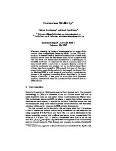
Note that stack 1 has been split into stack 1 0 and stack 1 1, and similarly local 1 has been split into local 1 0 and local 1 1. This splitting is quite important, because a single local or stack location in the bytecode can refer to di�erent types at di�erent program points. A complete example of a Java program with it's untyped and typed Jimple code is shown in Figure 1. The typed version was computed using the algorithms presented in this paper. In reality, the stack analysis, the introduction of new local variables, and the transformation are not as straightforward as it looks here. This is due to the presence of subroutines (the jsr bytecode instruction) and double-word values (long, double). A complete description of the bytecode to Jimple transformation can be found in [9]. 2
2
import java.awt.*; class Test { static Component method(boolean b) { Component c = new Button(); if(b) { c = new Choice(); } Object o = c; o.notify(); return c; } }
(a) Original Java Program
class Test extends java.lang.Object { static java.awt.Component method(boolean param0) { unknown_type v0; unknown_type v1; unknown_type v2; unknown_type v3; v0 := param0; v1 = new java.awt.Button; specialinvoke v1.[void java.awt.Button.()](); v2 = v1; if v0 == 0 goto label0; v3 = new java.awt.Choice; specialinvoke v3.[void java.awt.Choice.()](); v2 = v3;
}
label0: virtualinvoke v2.[void java.lang.Object.notify()](); return v2; }
(b) Untyped Jimple
class Test extends java.lang.Object { static java.awt.Component method(boolean param0) { int v0; java.awt.Button v1; java.awt.Component v2; java.awt.Choice v3; v0 := param0; v1 = new java.awt.Button; specialinvoke v1.[void java.awt.Button.()](); v2 = v1; if v0 == 0 goto label0; v3 = new java.awt.Choice; specialinvoke v3.[void java.awt.Choice.()](); v2 = v3;
}
label0: virtualinvoke v2.[void java.lang.Object.notify()](); return v2; }
(c) Typed Jimple
Figure 1: Example of Typing Jimple 3
3 Problem Statement The type inference problem we want to solve is a yes/no problem. We want to know if there exists a static type assignment for all local variables such that all type restrictions imposed by Jimple instructions on their arguments are met. If the answer is yes, we want a certi cate; a proof in the form of a valid type assignment for the variables. In the case where there exist more than one solution, we only require one of these solutions. If there are no solutions, we want to get a no answer. The restrictions of Jimple instructions on the type of their arguments are the same as the static restrictions imposed by the bytecode instructions on their arguments. For example, an integer addition operator is not allowed to perform additions on variables of reference type, an assignment to a eld of type String cannot be made from a variable of type Object without a type cast, etc. As the static type of arguments and return values of a method called is explicitly included in a method invocation instruction 3 , the scope of our problem is reduced to a single method at a time. In other words, our analysis is intra-procedural. On the other hand, it requires some knowledge about the type hierarchy of the program. This knowledge is restricted to classes and interfaces explicitly referenced in the method body, and all their ancestor classes and interfaces. This is a relatively small set of classes in practice. Furthermore, the class hierarchy information can be cached between successive invocations of the type inference algorithm.
3.1 A restricted problem In the following sections (4 to 6), we will assume that the analyzed Jimple code contains no array instructions and no reference to array types. Furthermore, we will assume that there is a single integer type4 : int. All references to boolean, byte, short, char (in eld types and method signatures) are treated as int. This is similar to the semantics of Java bytecode. In section 7 we will lift the array type restriction, and discuss ways of handling integer types.
4 A Constraint System In this section, we transform the type inference problem stated in section 3.1 into a graph problem. The graph represents the constraints imposed on local variables by Jimple instructions in the body of an analyzed method. The constraint graph is a directed graph containing the following components: 1. hard nodes: each hard node has an explicit associated type. 2. soft nodes: each soft nodes represents a type variable. 3. directed edges: each edge represent a constraint between two nodes. 3 4
and because Java relies on static resolution of overloading, long is not an integer type, in our de nition.
4
A directed edge from node to node , represented in the text as � , means that should be assignable to b. The rules of assignment compatibility are explained in [7]. Simply stated, should be of the same type as , or should be a superclass (or superinterface) of . The graph is constructed via a single pass over the Jimple code, adding nodes and edges to the graph, as implied by each instruction. The collection of constraints is best explained by looking at a few representative Jimple statements. We will look at the simple assignment statement, the assignment of a binary expression to a local variable, and a virtual method invocation. All other constructions are similar. A simple assignment is an assignment between two local variables [ = ]. If variable is assigned to variable , the constraints of assignment compatibility imply that ( ) � ( ), where ( ) and ( ) represent the yet unknown respective types of and . So, in this case, we need to add two soft nodes ( ) and ( ), unless they are already present in the graph. We also need to add an edge from ( ) to ( ) (if not already present). The assignment of the following binary expression to local variable , [ = + 3], generates the following constraints: ( ) � ( ), ( ) � , and ( ) � . So we need to add at most one hard node, two soft nodes and three directed edges to the graph, as necessary. Our last and most complicated case is a method invocation, [ = ( )], or in full: a
b
a
b
a
a
b
b
a
b
b
T a
a
T a
T b
a
T a
T a
a
T b
b
T b
T b
a
T a
T b
T a
int
T b
a
b
int
a
b:equals c
a = virtualinvoke b.[boolean java.lang.Object.equals(java.lang.Object)] (c)
A method invocation carries much type information. So we get all the following constraints, each involving a hard node:
� ( ) � , because the return type of is , and we have a single integer type. � ( )� , from the declaring class of . � ( )� , from the argument type in the method signature. T a
int
equals
T b
java:lang:Object
T c
java:lang:Object
boolean
equals
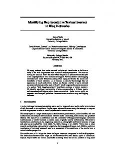
As usual, we must add all necessary edges and nodes to the constraint graph. Figure 2 shows the constraint graph of the example presented in Figure 1. Our type inference problem now consists of transforming soft nodes into hard nodes, such that all assignment compatibility constraints, represented by edges, are satis ed. If no such solution exists, or if a node needs more than one associated type, the type inference algorithm should report a no answer. We implement the graph using two adjacency lists on each node; a list of parents and a list of children. So, each directed edge is represented by two references, one parent and one child reference.
4.1 Complexity Analysis In this paper we do not present tight upper bounds on the running time of analyzes. We only take the necessary precautions to keep the worst case running cost of our fast algorithms below or equal to ( 2 ), where is the number of Jimple statements in the method body. It is important to note that the size of the constraint graph, [number of nodes]+[number of edges], is ( ). We will use this property throughout this paper. Our implementation uses e�cient data structures and O n
n
O n
5
Object
Component int
v0
v2
v1
Button
v3
Choice
Figure 2: Constraint Graph for Program in Figure 1 algorithms to keep the hidden constants as low as possible, or even reduce some costs to ( log ) or ( ). But as we will see in section 5.1, the dominating cost, that of merging, is ( 2 ) in the worst case. The worst case running time to decide whether a node or an edge is already present in the graph is ( ), where is the number of statements. Because the maximum number of edges and nodes added to the constraint graph is constant for each instruction, it follows that the upper bound on the running time of the graph construction algorithm is ( 2 ). O n
O n
O n
n
O n
n
O n
5 Solving Simple Constraints In this section, we describe three simple algorithms for reducing the number of soft nodes in the constraint graph built in section 4. This is achieved by merging adjacent nodes together. For each of these algorithm, we present a soundness proof and a worst running time analysis. But, rst, we introduce the merge operation and analyze, once and for all, its running time complexity. The three algorithms presented later should be applied consecutively, or more precisely in the order: rst, second, third and then second algorithm again. This is important for the validity of our soundness proofs.
6
5.1 Merging The main operation used by our simple algorithms is the merge operation. Two nodes are merged together whenever we can prove that: if there exists a non empty set of solutions to the type problem, then at least one of these solutions assigns the same type to both nodes. Merging has the nice property of reducing both the number of nodes and the number of edges in the constraint graph. But it must be done carefully. Merging consists of two parts. First, both nodes (or more precisely sets) are uni ed, then edges are combined. We use the fast union-set data structure [3]. Every time a merge is performed, the set representative is kept in the constraint graph, and all edges are xed to directly point to it. This give us the property that all merges are only done on set representatives, so the actual running time of the union operation is (1). (We need not pay for the more expensive nd operation).5 The cost of xing edges, on the adjacency list representation of the constraint graph, is the principal cost. Firstly, parents and children lists of merged nodes are combined, eliminating duplicates and references to both nodes. This can be done in ( ), by using a bit vector and adding the references one by one, setting a presence bit every time. Secondly, each child and parent node is visited once, replacing references to the eliminated node by references to the representative node (and avoiding duplicates). It is easy to see that each edge of the constraint graph won't be visited more than twice. So the total cost for one merge is ( ) + ( ) = ( ). The total number of nodes is ( ). The maximum number of merges that can be performed on the constraint graph is ( ) ? 1 = ( ). This gives us an upper bound of ( 2 ) on the total running time of all merges. We can now keep the cost of merges separate from the cost of other algorithms. This simpli es the remaining complexity analyzes. O
O n
O n
O n
O n
O n
O n
O n
O n
5.2 Solving Cyclic Constraints Our rst, and most simple transformation of the constraint graph, consists on nding cycles in the constraint graph, and then merging together all nodes of a cycle. Once cycles are removed, we are left with a dag (directed acyclic graph). We also take advantage of the veri er restrictions to merge respectively all values in a transitive relation with any of the non-reference basic type: int, long,
oat, and double. Figure 3 shows our previous constraint graph after applying this analysis. The soundness of rst part of this transformation is easy to establish6. If nodes are involved in a cycle 1 � 2 � � k � 1 , it follows that j � 1 for 2 = = by transitivity of �. But also, 1 � j , using the same argument. Therefore, 1 = j . It is then sound to assume that if there is a solution to the type problem, it will have the same type assignment for all 1 k nodes. The soundness of the second part is trivial. The algorithm used to detect cycles is the well known algorithm that nds strongly connected components in a directed graph [3]. The running time of this algorithm in linear in the size of the graph. This gives us ( ). This cost is e�ectively hidden by the cost of merges, in the overall worst case time analysis. Finding all nodes in a transitive relation with a basic type is also linear. (We start from the k
x
x
x
:::
x
x
x
x
x
x