Joint 48th IEEE Conference on Decision and Control and 28th Chinese Control Conference Shanghai, P.R. China, December 16-18, 2009
FrA17.5
Mean Square Stabilization of Multi-Input Systems over Stochastic Multiplicative Channels Nan Xiao, Lihua Xie and Li Qiu Abstract— This paper deals with the mean square stabilization problem for multi-input networked systems via single packet or multiple packets transmission, where the unreliability of input channels is modeled by a multiplicative white noise. For the single packet case, the critical value (lower bound) of mean square capacity for ensuring mean square stabilization is given by adopting the bisection technique. For the mparallel multiple packets transmission strategy, a necessary and sufficient condition on overall mean square capacity for mean square stabilization in terms of the Mahler measure or topological entropy of the plant is presented, under the assumption that the given network resource can be allocated among all the input channels. Applications in erasure-type channel and channel with stochastic sector-bounded uncertainty are provided to demonstrate the results.
I. I NTRODUCTION In the past few years, networked systems have found applications in a broad range of areas such as sensor networks, automated highway systems and unmanned aerial vehicles, due to their advantages over classical feedback control systems, e.g., low cost; flexibility; reduced weight and power requirement; simple installation and maintenance. However, networked systems require new formalisms for ensuring stability, performance and robustness, since in executing estimation and control operations, we cannot ignore the unreliability of network introduced by inherent computational and communication constraints. Therefore, significant research efforts have been and will continue to be devoted to this research area; see the survey papers [1], [2]. Several kinds of network uncertainties have been addressed in literature, for instance, packet dropout [3], [4], [5], quantization [6], [7], [8], time delay [9], and limited capacity [10], [11]. However, a unified treatment of these uncertainties is unavailable at present, although there are a few papers considering two or three issues mentioned above simultaneously, e.g., [12] for logarithmic quantization and binary i.i.d. packet loss; [13] for logarithmic quantization, bounded transmission delay and bounded packet dropout. The most pertinent results to this paper are [14] and [15]. Elia [14] considered the mean square stabilization over a fading channel in the framework of robust control, where This work was supported by Agency for Science, Technology and Research under Grant SERC 0521010037, NSFC of China under Grant 60828006, NSFC-Guangdong Joint Foundation U0735003, and Hong Kong Research Grants Council under GRF 618608. N. Xiao and L. Xie are with School of Electrical and Electronic Engineering, Nanyang Technological University, Singapore 639798, Singapore
[email protected];
[email protected]
L. Qiu is with Department of Electronic and Computer Engineering, Hong Kong University of Science and Technology, Kowloon, Hong Kong
[email protected]
978-1-4244-3872-3/09/$25.00 ©2009 IEEE
the randomness of the fading was interpreted as a stochastic model uncertainty. Several channels fit in this general fading model, such as memoryless multiplicative channel and Rice fading channel. Moreover the binary i.i.d. packet loss case falls into the channel with erasure property. One of the interesting discoveries is that for single-input systems, the minimum demand for mean square capacity assigned to the input can be presented in terms of the topological entropy of the plant. Recently, Gu and Qiu [15] found that subject to a total network resource constraint, the stabilization problem of a linear time-invariant discrete-time multi-input system with bounded time-varying sector-bounded uncertainties in the input channels can be solved analytically via a modified µ synthesis, and the solution is given in terms of the Mahler measure or topological entropy of the plant as well. Note that [15] only addresses the deterministic uncertainty case for multi-input systems, while [14] only discusses the minimum requirement of mean square capacity for the single-input case. It is also worth mentioning that random uncertainties are prominent in networked systems such as random packet losses and/or quantization errors with certain distribution, and stochastic descriptions of underlying uncertainties can lead to less conservative results based on the classical robust control theory. Therefore, this paper considers the mean square stabilization problem for multi-input systems across unreliable multiplicative channels described by stochastic uncertainties. The remainder of the paper is organized as follows. The problem is formulated in Section II. The mean square stabilization problem is discussed in Section III and Section IV for the single packet case and multiple packets transmission case, respectively. Applications and conclusions follow in Section V and Section VI. Notation: ≡ means ”defined as”. The superscript 0 denotes the transpose of vector or matrix. A−1 , ρ(A) and λui (A) represent the inverse, the spectral radius and an unstable eigenvalue of n×n square matrix A, accordingly the Mahler measure and Q the topological entropy of A are defined by M (A) ≡ i |λui (A)| and H(A) ≡ ln M (A), respectively. When X and Y are real symmetric matrices, the notation X ≥ Y (respectively, X > Y ) indicates that X − Y is positive semidefinite (positive definite). I is the identity matrix, and 0 denotes the zero matrix or zero vector. Furthermore, let E(·) stand for the mathematical expectation operator. kG(z)k2 represents the traditional H2 -norm for transfer function matrix G(z). ⊗ denotes a Kronecker product, and vec(X) is the vector formed by stacking the columns of X into one long vector.
6893
FrA17.5 II. P ROBLEM F ORMULATION The overall system structure considered in this paper is depicted in Fig. 1.
Fig. 1. nels.
Remark 2.1: Note that the above model can describe communication network uncertainties including quantization [7], signal distortion [11] and packet dropouts [3]. In particular, for the logarithmic quantizer considered in [7], ξ(t) is a sector bounded time-varying gain, which is used to model a sector bounded nonlinear function of v(t). In [3], ξ(t) is a 0-1 binary valued variable/matrix which models a packetloss phenomenon. (4) can also be used to model the case where quantization and packet loss exist simultaneously, see Corollary 5.3 in this paper. In view of (4), the closed-loop system can be written as x(t + 1) = Ax(t) + Bξ(t)v(t).
Multi-Input Networked Control System over Multiplicative Chan-
(5)
Gu and Qiu [15] adopts ξ(t) = diag {1 + ∆1 (t), 1 + ∆2 (t), · · · , 1 + ∆m (t)} (6)
Consider a discrete-time multi-input LTI plant as follows: x(t + 1) = Ax(t) + Bu(t),
(1)
where x(t) ∈ Rn is the state, u(t) ∈ Rm is the control input. We will denote this system by (A, B) for simplicity. Assume that A is unstable, (A, B) is stabilizable and B = [B1 B2 · · · Bm ] has full-column rank. For any stabilizable pair (A, B), the following Wonham decomposition [16] will play a crucial role in our further deduction: b1 ? · · · ? A1 ? · · · ? 0 b2 · · · ? 0 A2 · · · ? ¯= , B A¯ = . . . .. .. . . .. (2) . . . . . .. .. . . .. 0 0 · · · Am
0 0 · · · bm
with ? representing the part which will not be used in the derivation and m X Ai ∈ Rni ×ni , bi ∈ Rni ×1 , ni = n, i=1
¯ = T −1 B with T1 being a similarity where A¯ = T1−1 AT1 , B 1 transformation matrix and each pair (Ai , bi ) stabilizable. In fact, the canonical form (2) reveals certain structure property of plant (1) with respect to each input channel. Another linear coordinate transformation involved in this paper is shown as follow: · ¸ · ¸ As 0 Bs −1 −1 ˜ ˜ A = T2 AT2 = , B = T2 B = , (3) 0 Au Bu where T2 is invertible, As is stable, all the poles of Au are unstable and (Au , Bu ) is controllable. Suppose x(t) is available at the controller, and the state feedback v(t) = Kx(t) is adopted throughout this paper. The control signal v(t) is then processed (e.g. quantized) and sent through a communication channel to the actuator. The above processing and communication are modeled by the following memoryless multiplicative form: u(t) = ξ(t)v(t),
with ∆i (t) ∈ [−δi , δi ], i = 1, 2, · · · , m representing quantization errors, which is a possibly nonlinear, time-varying, dynamic uncertain system, and presents the theorem below. Theorem 2.1: For a multiplicative channel described by (4) and (6), there exists aQnetwork resource allocation m ¯ {δ1 , δ2 , · · · , δm } satisfying i=1 δi = δ such that the networked system (5) is stabilizable if and only if 1 . (7) δ¯ < M (A) However, when the network uncertainties become stochastic, we need to establish a parallel result in stochastic scenario as shown in the following two sections, where both the single packet transmission and multiple packets transmission strategies will be considered. Before closing this section, let us recall the definition of mean square stability [14] and some useful results in matrix theory [17], [18]. Definition 2.1: For stochastic system x(t + 1) = h(x(t), ξ(t)), h(0, ·) = 0
(8)
with random process ξ(t) and possibly nonlinear mapping h(·, ·), the equilibrium point at the origin is mean square stable if for any given initial state x(0), M (t) ≡ E[x(t)x0 (t)] is well-defined for any t ≥ 0, and limt→+∞ M (t) = 0. Remark 2.2: Note that at every time step t, ξ(t) in (8) can be a continuous, or discrete, or even hybrid random variable/vector/matrix. Lemma 1: The statements below are true. (i) The matrix equation Y = M XN can be written in a vector form: vec(Y ) = (N 0 ⊗ M )vec(X). (ii) The matrix inversion lemma: for Y = X +M QN , and X, Y, Q nonsingular, Y −1 = X −1 − X −1 M (Q−1 + N X −1 M )−1 N X −1 . (iii) det(I + M N ) = det(I + N M ). (iv) The Hadamard’s inequality: for any m × m positive definite matrix Q = [qij ],
(4)
where ξ(t) is a deterministic function or a random process with certain distribution.
6894
det(Q) ≤
m Y
qii .
i=1
Furthermore, equality holds if and only if Q is diagonal.
FrA17.5 III. M EAN S QUARE S TABILIZATION VIA S INGLE PACKET T RANSMISSION In this section, we assume that at each time step t, all elements of v(t) ∈ Rm are packed into a single packet and then sent through the unreliable network. Assumption 3.1: Suppose ξ(t) in (5) is a white random variable with mean µ ≡ E{ξ(t)} 6= 0 and variance σ 2 ≡ E{(ξ(t) − µ)2 } < +∞. For a single multiplicative input/output channel, e.g., setting m = 1 in (1), Elia [14] presents the (normalized) mean square capacity as µ ¶ 1 µ2 2 CMS = fMS (µ, σ ) ≡ ln 1 + 2 . (9) 2 σ Adopt this definition of CMS for our single packet transmission, and further denote µ2 g = f (µ, σ 2 ) ≡ 1 + 2 . (10) σ Note that the larger the g, the larger the CMS . The next lemma summarizes a series of conditions for mean square stabilization. Lemma 2: Under Assumption 3.1, the following statements are equivalent. (i) System (5) or (A, B) over the network (4) is mean square stabilizable. (ii) There exists a state feedback gain matrix K such that ρ(Ψ) < 1, where Ψ = (A + µBK) ⊗ (A + µBK) + σ 2 BK ⊗ BK.
Further, if B is rank one, i.e., m = 1, then gc = M (A)2 ; if B is square and invertible, i.e., m = n, then gc = ρ(A)2 . Proof: First, the equivalence between (11) and (13) follows from the Schur complement decomposition with S = P −1 /µ, Y = KP −1 . Note that if (13) is true for g = ga > 1, then it holds for any g = gb ≥ ga . In this situation the bisection method can be used. The range of gc as well as the results on the two special cases can be found in Lemma 5.4 of [2]. In contrast to the multiplicative model (4) adopted in this paper, Braslavsky etc. [11] considers the additive white Gaussian noise (AWGN) channel with an input power constraint for single-input systems, i.e., u(t) = v(t) + n(t), where n(t) is a zero mean Gaussian white noise with variance σ 2 . The capacity of the AWGN channel is 1 log2 (1 + SNR). (14) 2 As stated in Theorem III.1 of [11], the lower bound of SNR in (14) for state feedback stabilization can be given by the Mahler measure of system matrix A, similar to the result in Proposition 3.1 for m = 1. Remark 3.1: Except for some special cases as shown in Proposition 3.1, the critical value gc is, in general, not connected with system matrix A explicitly, instead a bisection technique is needed. While this situation can be avoided if the network resource is allocatable among all input channels as presented in the next section. C≡
IV. M EAN S QUARE S TABILIZATION VIA m-PARALLEL PACKETS T RANSMISSION
(iii) There exist P > 0 and K such that P > (A + µBK)0 P (A + µBK) + σ 2 K 0 B 0 P BK. (11)
Now, each element of the state feedback signal v(t) is assumed to be sent through an independent multiplicative (iv) There exists P > 0 such that channel at every time step. 2 Assumption 4.1: In this section, we make the following µ A0 P B(B 0 P B)−1 B 0 P A. (12) two assumptions. P > A0 P A − 2 2 σ +µ In this situation, one possible state feedback gain can (A1) m-parallel channels: ξ(t) in (5) is a random matrix µ 0 −1 0 consisting of diagonal white noise process elements be chosen as K = KM ≡ − σ2 +µ B P A. 2 (B P B) (v) (Au , Bu ) over the network (4) with Au , Bu being ξ(t) = diag {ξ1 (t), ξ2 (t), · · · , ξm (t)} (15) defined in (3) is mean square stabilizable. Proof: See the Appendix. with mean µi ≡ E{ξi (t)} 6= 0 and variance σi2 ≡ We can further deduce the following result. E{(ξi (t) − µi )2 } < +∞. Proposition 3.1: Under Assumption 3.1, networked sys- (A2) The overall network resource constraint is given in tem (5) is mean square stabilizable if and only if the mean terms of capacity of the input channel is greater than some critical m X value, i.e., ¯ CMS = CMSi , CMSi = fMS (µi , σi2 ), CMS > CMSc , or g > gc , i=1 where CMSc = 12 ln(gc ), and gc ∈ [ρ(A)2 , M (A)2 ] can be obtained by applying the bisection method to the optimization below gc ≡ min g, g ∈ [ρ(A)2 , M (A)2 ] S>0,Y q 1 −S (AS + BY )0 ( g−1 BY )0 < 0. (13) AS + BY −S 0 s.t. q 1 BY 0 −S g−1
i.e., g¯ =
m Y
gi , gi = f (µi , σi2 ),
i=1
and furthermore {g1 , g2 , · · · , gm } can be allocated among the m-parallel channels. Remark 4.1: The overall constraint on the sum of CMSi in Assumption 4.1(A2) is reasonable, since CMSi is related to the bit rate of the i-th channel.
6895
FrA17.5 Let
where
˜ i (t) ≡ ξi (t) − µi . ∆ σi
© ª 2 0 Bm P Bm J = diag σ12 B10 P B1 , σ22 B20 P B2 , · · · , σm +Bµ0 P Bµ .
˜ i (t) has zero mean and unit variance. Based on the Then ∆ framework of fading channel studied in [14], we rewrite (5) as follows x(t + 1) = (A + Bµ K)x(t) + Bµ Φw(t) z(t) = Kx(t) ˜ w(t) = ∆(t)z(t)
(16) (17) (18)
where Bµ = Bdiag {µ1 , µ2 , · · · , µm } = [µ1 B1 µ2 B2 · · · µm Bm ], ½ ¾ σ1 σ2 σm Φ = diag , ,··· , µ1 µ2 µ r m r ¾ ½r 1 1 1 , ,··· , , = diag g1 − 1 g2 − 1 g −1 n o m ˜ ˜ 1 (t), ∆ ˜ 2 (t), · · · , ∆ ˜ m (t) . ∆(t) = diag ∆ Note that the stabilizability of (A, B) guarantees that of ˜ the mean network (setting ∆(t) = 0), i.e., (A, Bµ ) is stabilizable, as µi 6= 0 for every i = 1, 2, · · · , m. The transfer function from w(t) to z(t) of the mean network is denoted by G(z) ≡ K(zI − A − Bµ K)−1 Bµ Φ.
(19)
Lemma 3: Under Assumption 4.1, the following statements are equivalent. (i) System (5) or (A, B) over the network (4) is mean square stabilizable. (ii) There exists a diagonal scaling matrix D ∈ Rm×m such that inf
D>0, Diag.
kD−1 G(z)Dk2MS < 1,
In this situation, one possible state feedback gain can be chosen as K = KM ≡ −J −1 Bµ0 P A. (vi) (Au , Bu ) over the network (4) with Au , Bu being defined in (3) is mean square stabilizable. Proof: (i)⇔(ii): It follows from Theorem 6.4 in [14]. The rest of the results can be proved similarly to Lemma 2. The theorem below fully characterizes the relationship between the overall mean square capacity and the topological entropy of system matrix A for ensuring mean square stability of (5). Theorem 4.1: Under Assumption 4.1, there exists a network resource allocation {g1 , g2 , · · · , gm } such that the networked system (5) is mean square stabilizable if and only if g¯ > M (A)2 , (23) i.e., ¯ MS > H(A). C (24) Proof: In view of the equivalence between (i) and (vi) in Lemma 3, we assume that all the eigenvalues of A are either on or outside the unit circle without loss of generality. ⇒: First, by applying the matrix inversion lemma on (22), we have P −1 < (A0 P A)−1 + (A0 P A)−1 A0 P Bµ © ª−1 2 0 ×diag σ12 B10 P B1 , σ22 B20 P B2 , · · · , σm Bm P Bm ×Bµ0 P A(A0 P A)−1
(20)
where the mean square norm of G(z) with dimension m ×q m is defined as kG(z)kMS ≡ Pm 2 maxi=1,2,··· ,m j=1 kGij (z)k2 . 0 0 0 0 (iii) There exists K = [K1 K2 · · · Km ] such that ρ(Ψ) < 1, where
0−1 = A−1 P −1 + A−1 B ½A ¾ g1 − 1 g2 − 1 gm − 1 ×diag , , · · · , B 0 A0−1 0 PB B10 P B1 B20 P B2 Bm m m X (gi − 1)Bi Bi0 0−1 A , = A−1 P −1 A0−1 + A−1 Bi0 P Bi i=1
and hence
Ψ = (A + Bµ K) ⊗ (A + Bµ K) +
m X
Ã
det(P −1 ) < det(A−1 ) det I + σi2 Bi Ki
⊗ Bi Ki .
(v) There exists P > 0 such that P > A0 P A − A0 P Bµ J −1 Bµ0 P A,
(22)
i
i=1
0 0 ] such (iv) There exist P > 0 and K = [K10 K20 · · · Km that
i=1
!
Bi0 P Bi
× det(P −1 ) det(A0−1 ) ¡ ¢ ¯ 0P B ¯ = det(A−1 )2 det(P −1 ) det I + B (25) m Y ≤ det(A)−2 det(P −1 ) gi (26)
i=1
P > (A + Bµ K)0 P (A + Bµ K) m X + σi2 Ki0 Bi0 P Bi Ki .(21)
m X (gi − 1)Bi B 0 P
i=1
= M (A)−2 det(P −1 )¯ g, where (25) is due to (iii) of Lemma 1 and s s "s # g − 1 g − 1 g − 1 1 2 m ¯= B1 B2 · · · Bm . B 0 PB B10 P B1 B20 P B2 Bm m
6896
FrA17.5 In the above, inequality (26) follows from the positive ¯ 0P B ¯ and the Hadamard’s inequality. definiteness of I + B Thus, we can conclude that g¯ > M (A)2 . ⇐: A constructive proof will be given by adopting a similar technique in [15]. According to (2), with the same ¯ B ¯µ ) and T1 , (A, Bµ ) has the Wonham decomposition (A, ¯b1 ? · · · ? 0 ¯b2 · · · ? ¯µ = T −1 Bµ = B (27) .. .. . . .. 1 . . . . 0 0 · · · ¯bm with ¯bi = µi bi and each pair (Ai , ¯bi ) controllable. Choose D = diag{1, ², · · · , ²m−1 } with a small real number ² > 0 and define S = diag{In1 , ²In2 , · · · , ²m−1 Inm }. ˆ ≡ KT1 and let K ˆ have the blockNow, we denote K ˆ = diag{k1 , k2 , · · · , km }, ki ∈ R1×ni , diagonal form K such that Ai + ¯bi ki is stable and thus, according to Corollary 8.4 in [14], we can get inf kki (zI − Ai − ¯bi ki )−1¯bi k22 = M (Ai )2 − 1. ki
Since
(28)
A1 o(²) · · · o(²) 0 A2 · · · o(²) ¯ = Aˆ = S −1 AS .. .. . . .. , . . . . 0 0 · · · Am ¯b1 o(²) · · · o(²) 0 ¯b2 · · · o(²) ˆµ = S −1 B ¯µ D = B .. .. . . .. , . . . . 0 0 · · · ¯bm ˆ = D−1 KT1 S, K
The equivalence between (23) and (24) is obvious based on expressions (9)(10). This completes the proof. V. A PPLICATIONS In this part, we only consider the m-parallel transmission strategy, while the single packet case can be addressed analogously via Proposition 3.1. A. Capacity Constraint Induced by Packet Loss Assumption 5.1: Suppose corresponding to the i-th channel, i = 1, 2, · · · , m, the packet-loss process is driven by an i.i.d. random variable θi (t) with probability distribution Pr{θi (t) = 0} = αi , Pr{θi (t) = 1} = 1 − αi , 0 ≤ αi < 1. (29) We have ξ(t) = diag {θ1 (t), θ2 (t), · · · , θm (t)} with µi = 1 − αi , σi2 = αi (1 − αi ), and hence gi = αi−1 . Theorem 4.1 gives us the following corollary. Corollary 5.1: Under Assumptions 4.1 and 5.1 there exists Qm a data loss rate allocation {α1 , α2 , · · · , αm } satisfying ¯ such that the networked system (5) is mean i=1 αi = α square stabilizable if and only if α ¯ < M (A)−2 . Obviously, the above corollary is consistent with the result of [2] if m = 1. B. Capacity Constraint Induced by Random Sector-Bounded Uncertainty
we have D−1 G(z)D = D−1 K(zI − A − Bµ DD−1 K)−1 Bµ DΦ ¯ − S −1 B ¯µ DD−1 KT1 S)−1 = D−1 KT1 S(zI − S −1 AS −1 ¯ ×S Bµ DΦ ˆ ˆµ K) ˆ −1 B ˆµ Φ = K(zI − Aˆ − B r r ½ 1 1 = diag G1 (z) , G2 (z) ,··· , g1 − 1 g2 − 1 r ¾ 1 Gm (z) + oz (²), gm − 1 where Gi (z) = ki (zI − Ai − ¯bi ki )−1¯bi , and oz (²) is a function of ² as well as z satisfying lim²→0 oz (²) = 0. Qm For g¯ > M (A)2 = i=1 M (Ai )2 , we can always choose gi > M (Ai )2 and ki according to (28), such that kGi (z)k22 < 1, for ∀i = 1, 2, · · · , m. gi − 1 It follows that kD−1 G(z)Dk2MS < 1 for sufficiently small ², i.e., there exist a positive diagonal matrix D, a stabilizing ˆ −1 state Qm feedback gain K = KT1 and a factorization g¯ = i=1 gi such that system (5) is mean square stable.
Assumption 5.2: Revisit the multiplicative channels modeled by (6), but now ∆i (t) is assumed to be uniformly distributed over [−δi , δi ] for every i = 1, 2, · · · , m and t. See [8] for a similar model of single logarithmic-quantized input. Then, µi = 1, σi2 = 13 δi2 , gi = δ32 + 1. i Corollary 5.2: Under Assumptions 4.1 and 5.2 there exists a network resource allocation {δ1 , δ2 , · · · , δm } satisfying ´ Qm ³ 3 + 1 = g ¯ such that the networked system (5) is 2 i=1 δi mean square stabilizable if and only if g¯ > M (A)2 . (30) Other than uniform distribution, any other type of distribution with constant expectation and variance can be adopted for ξi (t) or ∆i (t). By taking the stochastic information into account, less conservative results can be obtained; see the differences between Corollary 5.2 and Theorem 2.1, as the ¯ < M 1(A) . condition (30) can be rewritten as √Qm δ 2 i=1 (3+δi )
It is also easy to extend the above results to more complicated situations by choosing ξ(t) in (5) appropriately, e.g., combining the above packet loss case and sector-bounded uncertainty case together by setting ξi (t) = θi (t)(1+∆i (t)). Corollary 5.3: Suppose the m-parallel channels (15) is described by ξi (t) = θi (t)(1+∆i (t)), where θi (t) is i.i.d. satisfying (29) and ∆i (t) is uniformly distributed over [−δi , δi ], then under Assumption 4.1 there exists a network resource allocation {α , α , · · · , αm } and {δ1 , δ2 , · · · , δm } satisfying Qm ³ 3+δi21 ´ 2 = g¯ such that the networked system (5) is i=1 3αi +δi2 mean square stabilizable if and only if g¯ > M (A)2 .
6897
FrA17.5 VI. C ONCLUSIONS In this paper, the overall minimal mean square capacity for guaranteeing the mean square stabilization is given for a multi-input system with multiplicative input channels described by white processes. It is direct to generalize the results in this paper to observer design over unreliable multioutput channels via the duality. However, the corresponding Kalman filtering and LQG control problems are not so straightforward and would be interesting topics worth of investigation. Considering multiplicative channel with both stochastic and deterministic uncertainty also deserves future studies, where preliminary results on single-input case can be found in [12], [19]. A PPENDIX I P ROOF OF L EMMA 2 (i)⇔(ii): Based on Definition 2.1, we can obtain M (t + 1) = E[(Ax(t) + Bξ(t)Kx(t))(Ax(t) + Bξ(t)Kx(t))0 ] = (A + µBK)M (t)(A + µBK)0 + σ 2 BKM (t)K 0 B 0 . It then follows from (i) of Lemma 1 that vec(M (t + 1)) = Ψvec(M (t)) = Ψt+1 vec(M (0)). Thus, the mean square stabilization of (5) is equivalent to the existence of K such that ρ(Ψ) < 1, following the argument in Lemma 2 of [4]. (i)⇔(iii): It can be proved following a similar line of the proof on page 136-137 of [20]. (iii)⇐(iv): Inequality (12) implies that (11) is true by setting K = KM . (iii)⇒(iv): By taking derivative, it is easy to get that u = Kx = KM x minimizes the following function Θ ≡ −x0 P x + (Ax + µBu)0 P (Ax + µBu) + σ 2 u0 B 0 P Bu, which completes the proof. (i)⇐(v): Since As in (3) is stable, there exists P1 such that P1 − A0s P1 As > 0. (Au , Bu ) over (4) is mean square stabilizable, thus based on condition (iii) there exist P2 and Ku such that P2 > (Au +µBu Ku )0 P2 (Au +µBu Ku )+σ 2 Ku0 Bu0 P2 Bu Ku , which further implies that for some β > 0 P2 > βI + (Au + µBu Ku )0 P2 (Au + µBu Ku ) +σ 2 Ku0 Bu0 P2 Bu Ku . Denote Q ≡ Ku0 Bs0 P1 Bs Ku − Ku0 Bs0 P1 As (P1 − A0s P1 As )−1 A0s P1 Bs Ku . By choosing a sufficiently large γ > 0 such that γβI − Q > 0, we can get ˜ K) ˜ 0 P˜ (A˜ + µB ˜ K) ˜ + σ2 K ˜ 0B ˜ 0 P˜ B ˜ K, ˜ P˜ > (A˜ + µB ˜ B ˜ are defined as in (3), P˜ = diag{P1 , γP2 } where A, ˜ = [0 Ku ]. Further, it is immediate to prove that and K the mean square stabilizability is invariant under similarity transformations. This completes the proof.
˜ = (i)⇒(v): There exist P˜ = [P˜1 P˜3 ; P˜30 P˜2 ] and K ˜ ˜ [Ks Ku ] such that ˜ K) ˜ 0 P˜ (A˜ + µB ˜ K) ˜ + σ2 K ˜ 0B ˜ 0 P˜ B ˜ K. ˜ P˜ > (A˜ + µB (31) After applying the linear coordinate transformation matrix T3 = [I − P˜1−1 P˜3 ; 0 I], it is direct to deduce P2 > (Au +µBu Ku )0 P2 (Au +µBu Ku )+σ 2 Ku0 Bu0 P2 Bu Ku from the 2 × 2 block of the inequality (31), where P2 = ˜u − K ˜ s P˜ −1 P˜3 . Therefore, P˜2 − P˜30 P˜1−1 P˜3 > 0, Ku = K 1 (Au , Bu ) over (4) is mean square stabilizable. R EFERENCES [1] W. Zhang, M. Branicky, and S. Phillips, “Stability of networked control systems,” IEEE Control Systems Magazine, vol. 21, no. 1, pp. 84–99, 2001. [2] J. P. Hespanha, P. Naghshtabrizi, and Y. Xu, “A survey of recent results in networked control systems,” Proceedings of the IEEE, vol. 95, no. 1, pp. 138–162, 2007. [3] B. Sinopoli, L. Schenato, M. Franceschetti, K. Poolla, M. Jordan, and S. Sastry, “Kalman filtering with intermittent observations,” IEEE Transactions on Automatic Control, vol. 49, no. 9, pp. 1453–1464, 2004. [4] S. Hu and W. Yan, “Stability robustness of networked control systems with respect to packet loss,” Automatica, vol. 43, no. 7, pp. 1243–1248, 2007. [5] N. Xiao, L. Xie, and M. Fu, “Kalman filtering over unreliable communication networks with bounded Markovian packet dropouts,” In Press, International Journal of Robust and Nonlinear Control, DOI: 10.1002/rnc.1389, 2008. [6] N. Elia and S. Mitter, “Stabilization of linear systems with limited information,” IEEE Transactions on Automatic Control, vol. 46, no. 9, pp. 1384–1400, 2001. [7] M. Fu and L. Xie, “The sector bound approach to quantized feedback control,” IEEE Transactions on Automatic Control, vol. 50, no. 11, pp. 1698–1711, 2005. [8] T. Qi and W. Su, “Optimal tracking design for a linear system with a quantized control input,” in Proceedings of the 27th Chinese Control Conference, 2008, pp. 437–441. [9] J. Nilsson, “Real-Time Control Systems with Delays,” Lund, Sweden: Lund Institute of Technology, 1998. [10] A. Sahai and S. Mitter, “The necessity and sufficiency of anytime capacity for stabilization of a linear system over a noisy communication link-part I: scalar systems,” IEEE Transactions on Information Theory, vol. 52, no. 8, pp. 3369–3395, 2006. [11] J. Braslavsky, R. Middleton, and J. Freudenberg, “Feedback stabilization over signal-to-noise ratio constrained channels,” IEEE Transactions on Automatic Control, vol. 52, no. 8, pp. 1391–1403, 2007. [12] H. Hoshina, K. Tsumura, and H. Ishii, “The coarsest logarithmic quantizers for stabilization of linear systems with packet losses,” in Proceedings of the 46th IEEE Conference on Decision and Control, 2007, pp. 2235–2240. [13] H. Gao and T. Chen, “H∞ estimation for uncertain systems with limited communication capacity,” IEEE Transactions on Automatic Control, vol. 52, no. 11, pp. 2070–2084, 2007. [14] N. Elia, “Remote stabilization over fading channels,” Systems & Control Letters, vol. 54, no. 3, pp. 237–249, 2005. [15] G. Gu and L. Qiu, “Networked stabilization of multi-input systems with channel resource allocation,” in Proceedings of the 17th IFAC World Congress, 2008, pp. 625–630. [16] W. Wonham, “On pole assignment in multi-input controllable linear systems,” IEEE Transactions on Automatic Control, vol. 12, no. 6, pp. 660–665, 1967. [17] R. Horn and C. Johnson, Matrix Analysis. Cambridge University Press, 1985. [18] ——, Topics in Matrix Analysis. Cambridge University Press, 1991. [19] N. Xiao, L. Xie, and M. Fu, “Quantized stabilization of markov jump linear systems via state feedback,” in Proceedings of American Control Conference, 2009, pp. 4020–4025. [20] S. Boyd, L. El Ghaoui, E. Feron, and V. Balakrishnan, Linear Matrix Inequalities in System and Control Theory. Society for Industrial Mathematics, 1994.
6898