arXiv:0801.0109v2 [physics.soc-ph] 19 May 2008
Meaning and Form in a Language Computer Simulation Søren Wichmann1,2 , Dietrich Stauffer3 , Christian Schulze3 , F. Welington S. Lima 4 , and Eric W. Holman5,6 . 1
Department of Linguistics, Max Planck Institute for Evolutionary Anthropology, Deutscher Platz 6, D-04103 Leipzig, Germany;
[email protected] 2
Faculty of Archaeology, Leiden University, P.O. Box 9515, 2300 RA Leiden, The Netherlands 3
Institute for Theoretical Physics, Cologne University, D-50923 K¨oln, Euroland 4
Departamento de F´ısica, Universidade Federal do Piau´ı, 54049-550 Teresina - PI, Brazil 5
Department of Psychology, University of California, Los Angeles, California 90095-1563, USA. 6
Authors are listed in inverse alphabetical order.
Abstract: Thousands of different forms (words) are associated with thousands of different meanings (concepts) in a language computer model. Reasonable agreement with reality is found for the number of languages in a family and the Hamming distances between languages.
1
Introduction
The competition between languages of adult people [1] has been intensively simulated on computers [2, 3] or mathematically [4] for several years. When language structures were studied, they usually consisted of about a dozen features, often binary [5, 6, 7]; see [8] for a review. This number corresponds roughly to the 47 statistically independent language features [9] in the World Atlas of Language Structures [10], which relate to phonology, morphology, and syntax. In contrast, thousands of words are needed in everyday life for thousands of different concepts, not counting special terms e.g. from the sciences. While the origin of words has already been simulated [11], we want to simulate the subsequent proliferation and competition between thousands of languages, each containing thousands of forms for thousands of meanings. In 1
addition we try to get realistic statistics for the number of language families containing a given number of languages, and for the similarity of languages within one family and between different families.
Histogram: F=Q=7000, tau=40, t=60, split=15%
frequency
10
1
0.1
1
10 size of family
100
Figure 1: Family size distributions. The symbols connected with lines correspond to the parameter settings in the headline, while those not connected with lines have F = Q = 2000 and t = 100. In both cases three samples are shown differing only in the random numbers. The slope of the straight line corresponds to the empirical power law of [14]; see also [15]. In the present paper we regard grammatically related words (e.g., life, live, lives, lived, living) as one ”form”, and denote similarly related concepts by one ”meaning”. In the terminology of linguistics this corresponds to looking only at lexical morphemes, ignoring various inflections and derivations. Thus our N languages consist each of F meanings and Q forms; each meaning i = 1, 2, . . . F is expressed by one form Si = 1, 2, . . . Q. One form may be associated to several meanings, but no meaning is associated to several forms. In reality the latter case, called homophony by linguists, does occur, but is somewhat rarer than the former case, termed polysemy. 2
Within (lower data) and between (higher data) families 80
70 60 50 40 30 20 10 0 40
50
60
70 time
80
90
100
Figure 2: Evolution of Manhattan Hamming distances for the simulations of Fig.1. The simulations up to 60 iterations refer to F = Q = 7000, those for t ≤ 100 to F = Q = 2000. See Fig.14 in [16] for similar results. The simulations allow for cases where a given meaning is not realised in a given language, taking into account the sensitivity of the lexical inventories of languages to differences in cultural and natural environments. Such an unrealized meaning could be denoted by Si = Q. We start with one language and one form, where all meanings have the central form Si = Q/2; thus both the initial evolution of languages and their later competition are simulated. Then we apply three processes: Change (”mutation”) and diffusion (”transfer”) of single features Si as in the Schulze model [8], plus splitting [12] and merging of whole languages. In this last (new?) process, two languages which agree in all their Si at one time are regarded as one language from then on, changing, diffusing, and splitting together, and potentially undergoing further merging with other languages. The real-world parallel to merging would be cases where incipient differences disappear shortly after they arise, something that happens when children 3
F=Q=7000,Lmax=70000,f=0.1,split=10(+),15(x),20(*)%
frequency
10 1 0.1 0.01 0.001 1
10
100 size of family
1000
Several samples, splitting probability 20 % 10
frequency
1 0.1 0.01 0.001 1
10
100 size of family
1000
Figure 3: Top: Three simulations with the modified definition of ”family”, the line corresponds to reality [14]. Bottom: Sample to sample fluctuations when only the random number seed is changed. change ”wrong” forms popular among their peers to grown-up ”correct” forms, when slang forms are invented and later forgotten again, when ingroup varieties emerge and disappear, or when speakers of dialects shift to the standard variety. Different from the Schulze model and more similar to the Viviane und Tuncay models [13, 12], we no longer simulate each individual but only the language as a whole. Thus the ”population” for one language no longer is part of this model, and therefore, in contrast to the Schulze model, we have no shift from languages spoken by few people to more widespread languages, only merging of similar variants, as mentioned above. And we cannot determine a language size distribution, only a distribution for the number of languages within one language family. Otherwise the new 4
Histogram of yes-no distances, same simulations 1M
number
100000 10000 1000 100 10 1 1
10 Hamming distance
100
Figure 4: Distribution of Hamming distances in the simulations of Fig.3 top. See Fig.14 in [16] for similar results. model is similar to the Schulze model. In the next section we define the parameters of this model, then present our results, and in section 4 offer some modifications..
2
Model
A ”language” is defined by a string of F forms Si , for each meaning i between 1 and F , where Si is an integer between 1 and Q. Thus QF different languages are possible. At each iteration t = 1, 2, . . . we go in the same order through all N(t) different languages existing at that time t. Each of the F language features at each iteration undergoes with probability p a change, which means with probability q it takes over the corresponding Si of a randomly selected language then existing in the model, and with probability 1 − q it changes its own Si by ±1 (but not below 1 or above Q). Also, at each iteration all language pairs agreeing in all their corresponding Si are merged into one 5
F=Q=7000, Lmax=70,000, split=f=10% 10000
languages
1000
100
10
1 0
20
40
60
80 100 120 140 160 time
Figure 5: Time variation of the number L of languages in one of the samples of Fig.3 top. language (N → N − 1), and all languages surviving this merging split with probability s into two languages (N → N + 1) which from then on may diverge through change (p) and diffusion (q). We start with N = 1 language and during the first τ iterations switch off the merging process (since otherwise we would always stay at one, albeit changing, language). At the end of this time lag t = τ each language is regarded as the founder of one language family, comprising e.g. all IndoEuropean languages. The ”size” of a family is the number of different languages in it, arising from the later splitting process. In this sense the model combines language evolution and language competition. A Fortran program is available upon request.
6
p=0.010;q=0.1(+),0.3(x),0.5(*),0.7(sq.),0.9(full sq.)
frequency
10 1 0.1 0.01 0.001 1
10
100 size of family
1000
p=0.001;q=0.1(+),0.3(x),0.5(*),0.7(sq.),0.9(full sq.)
frequency
10 1 0.1 0.01 0.001 1
10
100 size of family
1000
Figure 6: Modified family size distributions for various diffusion probabilities q, with p = 0.01 (top) and 0.001 (bottom); F = Q = 7000. The lines again indicate reality [14].
3
Results
Mostly we worked with 7000 meanings and 7000 forms, at p = 0.001, q = 0.9, s = 0.15, τ = 40, 102 iterations. Figure 1 shows the size distribution for the families, which seems to be log-normal (parabola in this log-log plot). The plot is based on about 6000 languages in about 500 language families which are realistic numbers [14] for the number of languages in the present world. But since the distribution is more log-normal than power-law, the largest real families with about 1000 languages are missing in this model. The Manhattan Hamming distance is the sum over all absolute differences between the corresponding Si of the two languages. Figure 2 gives the time 7
p = 0.010, q=0.1, 0.3, 0.5, 0.7, 0.9 (right to left) 100000
number
10000 1000 100 10 1 1000 Hamming distance (yes-no)
10000
Figure 7: Modified yes-no Hamming distance distributions for various diffusion probabilities q, with p = 0.01, F = Q = 7000. dependence of the average Manhattan Hamming distances within one family and between different families; the second one is about twice as large as the first one, which seems reasonable [17]. All our simulations are nonequilibrium ones except for the number of families: The number of languages and the Hamming distances increase with time.
4
Modifications
A better result for the family size distribution, but a worse one for the Hamming distances, is obtained by a different family definition: whenever a new language is formed due to the splitting process, with probability f = 0.1 it is regarded as the founder of a new language family, with all later offspring languages belonging to it as long as they do not found a new family. Then we see in Fig.3 a better straight line (power law), extending to larger family sizes and agreeing with reality [14]. The distributions of Hamming distances 8
look as before, Fig.4, but now due to the random definition of ”family” there is no major difference between Hamming distances within one and between different language families. In these simulations we adopted a Verhulst extinction probability L/Lmax for each language at each iteration, where L is the current number of languages and Lmax = 70, 000. As a result the number of languages may stabilise as in Fig.5, even though the Hamming distances still increase; the number of families is about 100. Fig.6 shows that variations on the change and diffusion probabilities p, q give roughly the same family size distributions, and Fig.7 shows the variation of the Hamming distance histogram. (The numbers of families with only few language is lower in the simulations of Figs. 4 and 7 than in reality; perhaps the simulations underestimate the extinctions of languages.) The merging process was introduced to achieve, without our Verhulst extinction, a stationary number of languages at long t and very small F and Q. For the large F, Q and small t used here this aim is not achievable. The family sizes without merging look similar (not shown). For small F = Q = 100, 200, 500 we made up to a million iterations and then see how the average Manhattan Hamming distance stabilises. Its yes-no variant, counting only the number of different forms and not the amount of their difference, gets close to its maximum value, Fig.8, for increasing time (with extinction and merging). In Fig. 9 we compare simulation results with empirical data from 859 languages collected as part of a project on automated lexicostatistics. For each language, a 40-word subset [18] of the Swadesh 100-word basic vocabulary list [19] was transcribed in a standard orthography [20]. The distance between any two languages was defined as the percentage of attested words on the list that fail to match according to objective rules [20]. The data are well fit by the simulation with a low diffusion probability, q = 0.1: real and simulated languages differ typically in about 97% of their words. (Only near 100 % simulations and reality differ, since very few simulated languages differ by 100 %. With much smaller F = Q = 50 this peak does not shift; with q = 0.01 the peak shifts to 98 %. Thus this discrepancy does not go away.) This result suggests that borrowing is not the source of most changes in basic vocabulary. The greater variability of the data relative to the simulation may be attributed to two factors: first, random sampling variability in the data, which are based on a 40-word sample from a much larger true number of words; and second, the fact that likelihood of words matching in the data 9
varies with the length of the words, while the simulation treats all words equally. Finally, the largest languages F = Q = 7000 used up to now are still smaller than the actual numbers of words used in normal speech (without technical expressions and names). With a larger computer memory of 8 Gigabytes, and weeks of continuous simulation time, up to 200,000 meanings and forms were simulated with p = 0.001, q = 0.1, f = s = 0.1, τ = 50, surpassing the 105 words learned by adulthood [21]. Fig.10a shows no significant changes in the scaled position of the maximum for the yes-no Hamming distance, when F = Q is increased (also for F = Q = 3000 and 65,000; not shown). Fig.10b shows the whole distributions of the unscaled yes-no Hamming distance at F = Q = 200, 000 for various times t; at the right end of the plot we see a single maximum at t = 104 , followed to its right by three peaks of decreasing height at t = 105 . Fig.10 thus confirms for larger F = Q what was seen already in Figs.8,9, that for long times t a Hamming distance close to but below 100 percent is reached for the peak position.
5
Summary
Our model allowed for the first time for the simulation of thousands of meanings and forms. The resulting family size distribution was (depending on definition) close to log-normal or close to the power law of reality [15, 14], with large fluctuations. The distribution of Hamming distances had a skewed and realistic shape. With one of the definitions, strong differences, as desired, were found between the Hamming distances of languages within one family and between different families. Acknowledgement We thank a referee for drawing our attention to ref.[21]. For their efforts in gathering and analyzing the empirical data plotted in Fig. 9, we would like to acknowledge the members of the Automatic Similarity Judgment Project, in alphabetical order: Dik Bakker, Cecil H. Brown, Pamela Brown, Hagen Jung, Robert Mailhammer, Andr´e M¨ uller, and Viveka Velupillai. (Holman and Wichmann are also part of this project). A list of languages used, a map of their distribution, references to data sources, and two papers [18, 20] can be accessed through the project web page: http://email.eva.mpg.de/∼wichmann/ASJPHomePage.htm. 10
References [1] Wichmann, Søren. 2008. The emerging field of language dynamics. Language and Linguistics Compass 2.3: 442-455 = arXiv:0801.1415. [2] Nettle, Daniel. 1999b. Using social impact theory to simulate language change. Lingua 108: 95-117. [3] Abrams, Daniel and Steven H. Strogatz. 2003. Modelling the dynamics of language death. Nature 424: 900. [4] Zanette, Dami´an H. 2008. Analytical approach to bit-string models of language evolution. International Journal of Modern Physics C 19: in press, issue 4. [5] Kosmidis, Kosmas, J.M. Halley and Panos Argyrakis. 2005. Language evolution and population dynamics in a system of two interacting species, Physica A, 353: 595-612. [6] Schw¨ammle, Veit. 2005. Simulation for competition of languages with an ageing sexual population, International Journal of Modern Physics C 16: 1519-1526. [7] Schulze, Christian and Dietrich Stauffer. 2005. Monte Carlo simulation of the rise and fall of languages. International Journal of Modern Physics C 16: 781-787. [8] Schulze, Christian, Dietrich Stauffer, and Søren Wichmann. 2008. Birth, survival and death of languages by Monte Carlo simulation. Communications in Computational Physics 3: 271-294. [9] Holman, Eric W. 2008. Approximately independent features of languages. International Journal of Modern Physics C 19.2: 215-220. [10] Haspelmath, Martin, Matthew Dryer, David Gil, and Bernard Comrie (eds.) 2005. The World Atlas of Language Structures. Oxford: Oxford University Press. [11] Baronchelli, Andrea, Vittorio Loreto and Luc Steels. 2008. In-depth analysis of the Naming Game dynamics: the homogeneous mixing case. International Journal of Modern Physics C 19: in press. 11
[12] Tuncay, C ¸ a˘glar. 2008. Model of World; her cities, languages and countries. International Journal of Modern Physics C 19.2: 471-484. [13] de Oliveira, Viviane M., Marcelo A. F. Gomes, and Ing Ren Tsang. 2006. Theoretical model for the evolution of the linguistic diversity. Physica A 361: 361-370; de Oliveira, Paulo Murilo, et al. 2007. Bit-strings and other modifications of Viviane model for language competition. Physica A 376: 609-616. and 2008. A computer simulation of language families. In press for Journal of Linguistics, arXiv:0709.0868. [14] Wichmann, Søren. 2005. On the power-law distribution of language family sizes. Journal of Linguistics 41: 117-131. [15] Zanette, Dami´an. 2001. Self-similarity in the taxonomic classification of human languages. Advances in Complex Systems 4: 281-286. [16] Sattah, Shmuel and Amos Tversky. 2005. Additive Similarity Trees. Psychometrika 42, 319-345. [17] Wichmann, Søren and Eric W. Holman. Forthcoming. Pairwise comparisons of typological profiles. For the proceedings of the conference Rara & Rarissima—Collecting and Interpreting Unusual Characteristics of Human Languages. Preprint: 0704.0071 on arXiv.org [18] Holman, Eric W., Søren Wichmann, Cecil H. Brown, Viveka Vilupillai, Andr´e M¨ uller, and Dik Bakker. 2008. Explorations in automated lexicostatistics. In press for Folia Linguistica. [19] Swadesh, Morris. 1955. Towards greater accuracy in lexicostatistic dating. International Journal of American Linguistics 21: 121 - 137. [20] Brown, Cecil H., Eric W. Holman, Søren Wichmann, and Viveka Velupillai. 2008. Automated classification of the World’s languages: A description of the method and preliminary results. In press for Sprachtypologie und Universalienforschung. [21] Bloom, P. 2000. How children learn the meaning of words. Cambridge: MIT Press.
12
! Equilibration for F = Q = 500, split = f = 10 %
Hamming distance
1000
100
10 100
1000
10000
100000
time Histogram at t/1000=0.1, 1, 10, 100 (left to right)
100000
number
10000 1000 100 10 1 1
10 100 Hamming distance (yes-no)
1000
Histogram part at t/1000 = 10(*),100(sq.),1000(full sq.)
100000
number
10000 1000 100 10 1 300
320
340
360
380
400
420
440
Hamming distance (yes-no)
Figure 8: Time variation in modified model of average Hamming (Manhattan) distance (top) and of Hamming distance distribution (centre and bottom) for small F = Q = 500. 13
t=1 million, p=0.01, q=0.9(left) and 0.1(right) 1M 100000
number
10000 1000 100 10 1 0
20 40 60 80 Hamming distance in percent
100
Figure 9: Comparison of the reality (+) of automated lexicostatistics [18, 20] with equilibrium simulations (yes-no; lines) for F = Q = 1000. Shorter simulations with only 100,000 and 300,000 iterations are not significantly different. Thus q ≤ 0.1 roughly agrees with the lexicostatistical results.
14
Scaled yes-no Hamming distance
F=Q= 10,000(+), 100,000(x), 200,000(*) 1 0.8 0.6 0.4 0.2 0 0
0.1
0.2 0.3 1/log_10(time)
0.4
0.5
F=Q=200,000; t/1000=0.1, 1, 10, 100 left to right 12000 10000
numbers
8000 6000 4000 2000 0 0
50000 100000 150000 yes-no Hamming distance
200000
Figure 10: Top: Position of the maximum in the distribution of the yes-no Hamming distance, scaled by the largest possible distance F , as a function of 1/log(t), for three large values of F = Q. Note the flattening for t > 104 . The bottom part shows the whole distributions for the largest F = Q = 200, 000 (unscaled yes-now Hamming distance); sometimes there is a single peak, sometimes there are several peaks close together.
15