Methods for Efficient Storage and Indexing in XML ... - Semantic Scholar

Methods for Efficient Storage and Indexing in XML Databases

by Kanda Runapongsa

A dissertation submitted in partial fulfillment of the requirements for the degree of Doctor of Philosophy (Computer Science and Engineering) in The University of Michigan 2003

Doctoral Committee: Assistant Professor Jignesh M. Patel, Chair Professor Hosagrahar V. Jagadish Professor Atul Prakash Professor Toby J. Teorey Associate Professor Dawn M. Tilbury

c

Kanda Runapongsa All Rights Reserved

2004

DEDICATION

This dissertation is dedicated to my mother.

ii

ACKNOWLEDGEMENTS

I would like to express my gratitude to all those who gave me the possibility to complete this thesis. I am deeply indebted to my advisor Prof. Jignesh M. Patel for his suggestions and guidance in doing research and writing this thesis. I am inspired by his encouragement to enhance the quality of the work. I also appreciate his teachings of research, writing, and presentation skills. He also provides financial support when I need it. Without him, I would not have been able to accomplish this thesis. I am greatly grateful to Prof. Toby J. Teorey for his help and support, especially in my first few years. Without him, I would not have been able to continue my graduate studies. I also feel grateful to Prof. H. V. Jagadish for his ideas and suggestions in developing the Michigan Benchmark and for giving me the opportunity to review papers that are related to my research. I would like to express my gratitude to Prof. Atul Prakash and Prof. Dawn M. Tilbury for their time and commitment to serving on my committee. I also would like to thank Mimi Adam and Andrew McClory for helping me to edit research papers and this thesis. I would like to thank the Thai government and the IBM Toronto laboratory for their financial support. I would also like to thank Kelly Lyons for always believing in me and giving me the opportunity to work at several IBM Research Centers. I would like to thank Sriram Padmanabhan and Rajesh Bordawekar for their suggestions and guidance in developing XIST. In addition, I would like to thank Amanjot S Khaira iii

and Robert Schloss for providing programs to collect XML data statistics. I feel grateful to Richard Hankins for providing the implementation of persistent hash index and B+tree index that I have used in my experiments. I also feel grateful to Shurug Al-Khalifa and Yun Chen for their time and effort in running the Michigan benchmark on a number of different databases. I also would like to thank Nuwee Wiwatwattana for reviewing some chapters of this thesis. I also would like to thank my colleagues in the database research group for their comments about my work and their friendship. Living apart from my family would be difficult if I did not have friends in the United of States. I especially thank Saowapak Sotthivirat for her generosity and friendship. I think of her like a sister whom I would like to cherish the friendship with for the rest of my life. I also would like to thank Virapat Tantayakom, Narinporn Pattaramanon, and Phongphaeth Pengvanich for their special friendship. I feel fortunate for knowing Jayada Boonyakiet who always listens to me and cares about me. I would like to thank Seksan Kiatsupaibul, Elena Yamaguchi, Panita Pongpaibool, Warinthorn Songkasiri, Patrawadee Prasangsit, and Hongsuda Tangmunarunkit for their friendship. My family has always been with me even though I live physically apart from them. Especially, I would like to give my special thank to my mother for her constant unconditional love and encouragement. It has always been my dream to be able to return her favors for everything that she has been given to me. I would like to thank my sisters, Kanokporn Wongkaew and Duangporn Runapongsa, for their genuine love and support. I also would like to thank Buddhadasa Bhikkhu for his teachings about the truth of life, and Dr. Prawase Wasi for his inspiring thoughts and actions in living a happy and meaningful life.

iv

TABLE OF CONTENTS

DEDICATION . . . . . . . . . . . . . . . . . . . . . . . . . . . . . . . . . .

ii

ACKNOWLEDGEMENTS . . . . . . . . . . . . . . . . . . . . . . . . . .

iii

LIST OF FIGURES . . . . . . . . . . . . . . . . . . . . . . . . . . . . . . .

ix

LIST OF TABLES . . . . . . . . . . . . . . . . . . . . . . . . . . . . . . . . xiv LIST OF APPENDICES . . . . . . . . . . . . . . . . . . . . . . . . . . . . xv CHAPTER I. Introduction . . . . . . . . . . . . . . . . . . . . . . . . . . . . . . 1.1 1.2

1

Research Issues and Contributions . . . . . . . . . . . . . . . Thesis Outline . . . . . . . . . . . . . . . . . . . . . . . . . .

4 7

II. Background . . . . . . . . . . . . . . . . . . . . . . . . . . . . . . .

9

2.1 2.2

. . . . . .

9 10 11 13 15 16

III. Storing and Querying Schema-based XML Documents Using an ORDBMS . . . . . . . . . . . . . . . . . . . . . . . . . . . . . .

17

2.3

3.1 3.2 3.3

Extensible Markup Language (XML) . . . . XML Schema Description Languages . . . . 2.2.1 Document Type Definition (DTD) 2.2.2 XML Schema . . . . . . . . . . . XML Query Languages . . . . . . . . . . . 2.3.1 XPath Expressions . . . . . . . .

. . . . . .

. . . . . .

. . . . . .

. . . . . .

. . . . . .

. . . . . .

. . . . . .

. . . . . .

. . . . . .

Introduction . . . . . . . . . . . . . . . . . . . . . . . . . . . Related Work . . . . . . . . . . . . . . . . . . . . . . . . . . . Storing XML Documents in an ORDBMS . . . . . . . . . . . 3.3.1 Reducing DTD Complexity . . . . . . . . . . . . . . 3.3.2 Building a DTD Graph . . . . . . . . . . . . . . . . 3.3.3 XORator: Mapping a DTD to an ORDBMS Schema 3.3.4 Defining an XML Data Type (XADT) . . . . . . . .

v

17 20 22 23 24 26 30

3.3.4.1 Storage Alternatives for the XADT . . 3.3.4.2 Functions on the XADT . . . . . . . . 3.3.5 An Unnest Operator . . . . . . . . . . . . . . . . . Performance Evaluation . . . . . . . . . . . . . . . . . . . . . 3.4.1 Implementation Overview . . . . . . . . . . . . . . . 3.4.2 Experimental Platform and Methodology . . . . . . 3.4.3 Experiments Using the Shakespeare Plays Data Set 3.4.4 Experiments Using the SIGMOD Proceedings Data Set . . . . . . . . . . . . . . . . . . . . . . . . . . . Conclusion and Future Work . . . . . . . . . . . . . . . . . .

44 51

IV. Storing and Querying XML Documents Using a Relational Database . . . . . . . . . . . . . . . . . . . . . . . . . . . . . . . . .

52

3.4

3.5

4.1 4.2

32 33 36 38 38 39 39

Introduction . . . . . . . . . . . . . . . . . . . . . . . . . . . Different Mapping Approaches . . . . . . . . . . . . . . . . . 4.2.1 The Begin-End-Level (BEL) Approach . . . . . . . 4.2.2 The Begin-End-Level-Path (BELP) Approach . . . 4.2.3 The Parent-ID (PAID) Approach . . . . . . . . . . Performance Evaluation . . . . . . . . . . . . . . . . . . . . . 4.3.1 Experimental Setup . . . . . . . . . . . . . . . . . . 4.3.2 Experiments Using the Shakespeare Plays Data Set 4.3.3 Experiments Using the SIGMOD Proceedings Data Set . . . . . . . . . . . . . . . . . . . . . . . . . . . Related Work . . . . . . . . . . . . . . . . . . . . . . . . . . . Conclusions . . . . . . . . . . . . . . . . . . . . . . . . . . . .

70 72 73

V. XIST: An XML Index Selection Tool . . . . . . . . . . . . . . .

75

4.3

4.4 4.5

5.1

5.2

5.3 5.4 5.5

5.6 5.7

Introduction . . . . . . . . . . . . . . . . . . . . . . . . . . . 5.1.1 Problem Statement . . . . . . . . . . . . . . . . . . 5.1.2 Contributions . . . . . . . . . . . . . . . . . . . . . Background . . . . . . . . . . . . . . . . . . . . . . . . . . . . 5.2.1 Models of XML Data, Schema, and Queries . . . . . 5.2.2 Terminologies and Assumptions . . . . . . . . . . . The XIST Algorithm . . . . . . . . . . . . . . . . . . . . . . . Candidate Path Selection . . . . . . . . . . . . . . . . . . . . Index Benefit Computation . . . . . . . . . . . . . . . . . . . 5.5.1 Cost-based Benefit Computation . . . . . . . . . . . 5.5.1.1 Computing Evaluation Costs . . . . . . 5.5.1.2 Using Cost Models for Computing Benefits 5.5.2 Heuristic-based Benefit Computation . . . . . . . . Configuration Enumeration . . . . . . . . . . . . . . . . . . . Experimental Evaluation . . . . . . . . . . . . . . . . . . . .

vi

52 54 56 57 61 65 66 66

75 77 78 79 79 81 83 86 89 90 91 92 94 96 97

5.7.1 5.7.2 5.7.3

5.8 5.9

Experimental Setup . . . . . . . . . . . . . . . . . . 97 Data Sets and Queries . . . . . . . . . . . . . . . . 98 Experimental Results . . . . . . . . . . . . . . . . . 99 5.7.3.1 Effectiveness of Path Equivalence Classes 99 5.7.3.2 Validation of the Cost Model . . . . . . 100 5.7.3.3 Comparison of Index Selection Techniques101 5.7.3.4 Impact of Input Information on XIST . 102 5.7.3.5 Impact of Changing Workloads on XIST 108 Related Work . . . . . . . . . . . . . . . . . . . . . . . . . . . 111 Conclusions . . . . . . . . . . . . . . . . . . . . . . . . . . . . 115

VI. The Michigan Benchmark . . . . . . . . . . . . . . . . . . . . . . 116 6.1 6.2 6.3

6.4

6.5

Introduction . . . . . . . . . . . . . . . . . . . . . . . . . . . 116 Related Work . . . . . . . . . . . . . . . . . . . . . . . . . . . 119 Benchmark Data Set . . . . . . . . . . . . . . . . . . . . . . . 121 6.3.1 A Discussion of the Data Characteristics . . . . . . 121 6.3.1.1 Depth and Fanout . . . . . . . . . . . . 121 6.3.1.2 Data Set Granularity . . . . . . . . . . . 122 6.3.1.3 Scaling . . . . . . . . . . . . . . . . . . 123 6.3.2 Schema of Benchmark Data . . . . . . . . . . . . . 124 6.3.3 String Attributes and Element Content . . . . . . . 125 Benchmark Queries . . . . . . . . . . . . . . . . . . . . . . . 128 6.4.1 Selection . . . . . . . . . . . . . . . . . . . . . . . . 129 6.4.1.1 Returned Structure . . . . . . . . . . . . 130 6.4.1.2 Selection on Values . . . . . . . . . . . . 131 6.4.1.3 Structural Selection . . . . . . . . . . . 131 6.4.2 Value-Based Join . . . . . . . . . . . . . . . . . . . 135 6.4.3 Pointer-Based Join . . . . . . . . . . . . . . . . . . 136 6.4.4 Aggregation . . . . . . . . . . . . . . . . . . . . . . 136 6.4.5 Update and Load . . . . . . . . . . . . . . . . . . . 137 6.4.6 Document Construction . . . . . . . . . . . . . . . . 137 The Benchmark in Action . . . . . . . . . . . . . . . . . . . . 138 6.5.1 Experimental Platform and Methodology . . . . . . 139 6.5.1.1 System Setup . . . . . . . . . . . . . . . 139 6.5.1.2 Data Sets . . . . . . . . . . . . . . . . . 140 6.5.1.3 Measurements . . . . . . . . . . . . . . . 141 6.5.1.4 Benchmark Results . . . . . . . . . . . . 141 6.5.2 Detailed Performance Analysis . . . . . . . . . . . . 143 6.5.2.1 Returned Structure (QR1-QR2) . . . . . 144 6.5.2.2 Exact Match (QS1-QS3) . . . . . . . . . 145 6.5.2.3 Approximate Match (QS4-QS5) . . . . . 146 6.5.2.4 Order-sensitive Selection (QS6-QS7) . . 146 6.5.2.5 Simple Containment Selection (QS8-QS13)147

vii

6.5.2.6

6.6

Complex Pattern Containment Selection (QS14-QS16) . . . . . . . . . . . . . . . 151 6.5.2.7 Irregular Structure (QS17) . . . . . . . . 151 6.5.2.8 Value-Based and Pointer-Based Joins (QJ1QJ4) . . . . . . . . . . . . . . . . . . . . 152 6.5.2.9 Aggregation (QA1-QA3) . . . . . . . . . 153 6.5.2.10 Update (QU1-QU3) . . . . . . . . . . . 154 6.5.2.11 Document Construction (QC1-QC2) . . 155 6.5.3 Performance Analysis on Scaling Databases . . . . . 156 6.5.3.1 Scaling Performance on CNX . . . . . . 156 6.5.3.2 Scaling Performance on Timber . . . . . 156 6.5.3.3 Scaling Performance on COR . . . . . . 156 Conclusions . . . . . . . . . . . . . . . . . . . . . . . . . . . . 157

VII. Conclusions and Future Work . . . . . . . . . . . . . . . . . . . 159 7.1 7.2

Conclusions . . . . . . . . . . . . . . . . . . . . . . . . . . . . 159 Future Work . . . . . . . . . . . . . . . . . . . . . . . . . . . 161

APPENDICES . . . . . . . . . . . . . . . . . . . . . . . . . . . . . . . . . . 163 BIBLIOGRAPHY . . . . . . . . . . . . . . . . . . . . . . . . . . . . . . . . 207

viii

LIST OF FIGURES

Figure 1.1

Methods in XML Databases that the Thesis Focuses on . . . . . . .

8

2.1

A Sample XML Document (bib.xml) . . . . . . . . . . . . . . . . .

9

2.2

A DTD of the Sample XML Document (bib.dtd) . . . . . . . . . . .

11

2.3

An XML Schema of the Sample XML Document (bib.xsd) . . . . .

14

3.1

A DTD of a Plays Data Set . . . . . . . . . . . . . . . . . . . . . .

23

3.2

A DTD of the Plays Data Set (Simplified Version) . . . . . . . . . .

24

3.3

The DTD Graph for the Plays DTD . . . . . . . . . . . . . . . . . .

25

3.4

The Revised DTD Graph for the Plays DTD . . . . . . . . . . . . .

25

3.5

The Overview of the XORator Algorithm . . . . . . . . . . . . . . .

28

3.6

The PostOrderTreeMapping Function . . . . . . . . . . . . . . . . .

29

3.7

The Relational Schema Transformed Using Hybrid . . . . . . . . . .

30

3.8

A DTD Graph When Using XORator . . . . . . . . . . . . . . . . .

31

3.9

Element Trees When Using XORator . . . . . . . . . . . . . . . . .

31

3.10

The Relational Schema Transformed Using XORator . . . . . . . .

32

3.11

Query QE1 in Both Algorithms . . . . . . . . . . . . . . . . . . . .

35

3.12

Query QE2 in Both Algorithms . . . . . . . . . . . . . . . . . . . .

35

3.13

Before and After Unnesting the speaker Attribute . . . . . . . . . .

37

ix

3.14

The DTD of the Shakespeare Data Set . . . . . . . . . . . . . . . .

40

3.15

Hybrid/XORator Performance Ratios on a Log Scale as Database Sizes Increase for the Shakespeare Data Sets . . . . . . . . . . . . .

43

Performance of Different Mappings for the Shakespeare DSx1 Data Set . . . . . . . . . . . . . . . . . . . . . . . . . . . . . . . . . . . .

44

Performance of Different Mappings for the Shakespeare DSx2 Data Set . . . . . . . . . . . . . . . . . . . . . . . . . . . . . . . . . . . .

45

Performance of Different Mappings for the Shakespeare DSx4 Data Set . . . . . . . . . . . . . . . . . . . . . . . . . . . . . . . . . . . .

45

3.19

The DTD of the SIGMOD Proceedings Data Set . . . . . . . . . . .

46

3.20

Hybrid/XORator Performance Ratios on a Log Scale as Database Sizes Increase for the SIGMOD Proceedings Data Sets . . . . . . . .

48

Performance of Different Mappings for the SIGMOD Proceedings DSx1 Data Set . . . . . . . . . . . . . . . . . . . . . . . . . . . . .

50

Performance of Uncompressed and Compressed Versions for the SIGMOD Proceedings DSx1 Data Set . . . . . . . . . . . . . . . . . . .

50

4.1

A Sample XML Document (with Word Positions in Bold) . . . . . .

55

4.2

The Element Relation of BEL . . . . . . . . . . . . . . . . . . . . .

57

4.3

The Text Relation of BEL . . . . . . . . . . . . . . . . . . . . . . .

58

4.4

A SQL Query When Using BEL . . . . . . . . . . . . . . . . . . . .

58

4.5

The Tree Structure in the Sample Document When Using BELP . .

60

4.6

The Element Relation of BELP . . . . . . . . . . . . . . . . . . . .

62

4.7

The Text Relation of BELP . . . . . . . . . . . . . . . . . . . . . .

62

4.8

The Path Relation of BELP . . . . . . . . . . . . . . . . . . . . . .

63

4.9

A SQL Query When Using BELP . . . . . . . . . . . . . . . . . . .

63

4.10

The Element Relation of PAID . . . . . . . . . . . . . . . . . . . . .

64

3.16

3.17

3.18

3.21

3.22

x

4.11

The Path Relation of PAID . . . . . . . . . . . . . . . . . . . . . .

64

4.12

The Text Relation of PAID . . . . . . . . . . . . . . . . . . . . . . .

65

4.13

A SQL Query When Using PAID (with Path Information) . . . . .

65

4.14

A SQL Query When Using PAID (with Element Name Information)

66

4.15

Other Approaches/PAID Performance Ratios on a Log Scale for the Shakespeare DSx1 Data Set . . . . . . . . . . . . . . . . . . . . . .

68

Other Approaches/PAID Performance Ratios on a Log Scale for the SIGMOD Proceedings DSx1 Data Set . . . . . . . . . . . . . . . . .

71

5.1

Sample XML Data . . . . . . . . . . . . . . . . . . . . . . . . . . .

81

5.2

Sample XML Schema . . . . . . . . . . . . . . . . . . . . . . . . . .

82

5.3

The XIST Architecture . . . . . . . . . . . . . . . . . . . . . . . . .

84

5.4

The XIST Algorithm . . . . . . . . . . . . . . . . . . . . . . . . . .

86

5.5

The Algorithm to Find Equivalence Classes (EQs) . . . . . . . . . .

88

5.6

The Index Benefit Computation Algorithm for CPI Ip . . . . . . . .

90

5.7

FE and FD for Ip (with Statistics) . . . . . . . . . . . . . . . . . . .

93

5.8

FE and FD for Ip (Without Statistics) . . . . . . . . . . . . . . . . .

95

5.9

Numbers of Paths and Equivalence Classes . . . . . . . . . . . . . . 100

5.10

Performance Improvement of XIST . . . . . . . . . . . . . . . . . . 102

5.11

Performance of Different Index Sets on DBLP (with Workload Information) . . . . . . . . . . . . . . . . . . . . . . . . . . . . . . . . 104

5.12

Performance of Different Index Sets on Mondial (with Workload Information) . . . . . . . . . . . . . . . . . . . . . . . . . . . . . . . . 105

5.13

Performance of Different Index Sets on Plays (with Workload Information) . . . . . . . . . . . . . . . . . . . . . . . . . . . . . . . . . 105

4.16

xi

5.14

Performance of Different Index Sets on XMark (with Workload Information) . . . . . . . . . . . . . . . . . . . . . . . . . . . . . . . . 106

5.15

Performance of Different Index Sets on DBLP (without Workload Information) . . . . . . . . . . . . . . . . . . . . . . . . . . . . . . . 107

5.16

Performance of Different Index Sets on Mondial (without Workload Information) . . . . . . . . . . . . . . . . . . . . . . . . . . . . . . . 108

5.17

Performance of Different Index Sets on Plays (without Workload Information) . . . . . . . . . . . . . . . . . . . . . . . . . . . . . . . 109

5.18

Performance of Different Index Sets on XMark (without Workload Information) . . . . . . . . . . . . . . . . . . . . . . . . . . . . . . . 109

5.19

Performance of Different Index Sets on DBLP (with Changing Workloads) . . . . . . . . . . . . . . . . . . . . . . . . . . . . . . . . . . 110

5.20

Performance of Different Index Sets on Mondial (with Changing Workloads) . . . . . . . . . . . . . . . . . . . . . . . . . . . . . . . 111

5.21

Performance of Different Index Sets on Plays (with Changing Workloads) . . . . . . . . . . . . . . . . . . . . . . . . . . . . . . . . . . 112

5.22

Performance of Different Index Sets on XMark (with Changing Workloads) . . . . . . . . . . . . . . . . . . . . . . . . . . . . . . . . . . 113

6.1

Distribution of the Nodes in the Base Data Set . . . . . . . . . . . . 123

6.2

Benchmark Specification in XML Schema . . . . . . . . . . . . . . . 126

6.3

The Template of a String Element Content . . . . . . . . . . . . . . 128

6.4

Samples of Chain and Twig Queries . . . . . . . . . . . . . . . . . . 134

6.5

Benchmark Numbers for the Three DBMSs . . . . . . . . . . . . . . 142

6.6

Benchmark Numbers of Returned Structure Queries . . . . . . . . . 144

6.7

Benchmark Numbers of Selection on Values Queries . . . . . . . . . 145

6.8

Benchmark Numbers of Approximate Match Queries . . . . . . . . . 146

6.9

Benchmark Numbers of Order-sensitive Queries . . . . . . . . . . . 147

xii

6.10

Benchmark Numbers of Structural Selection Queries . . . . . . . . . 148

6.11

Benchmark Numbers of Traditional Join Queries . . . . . . . . . . . 153

6.12

Benchmark Numbers of Aggregate Queries . . . . . . . . . . . . . . 154

6.13

Benchmark Numbers of Update Queries . . . . . . . . . . . . . . . . 155

6.14

Benchmark Numbers of Document Construction Queries . . . . . . 155

xiii

LIST OF TABLES

Table 3.1

Database Statistics for the Shakespeare DSx1 Data Set . . . . . . .

41

3.2

Execution Times of Hybrid and XORator for the Shakespeare DSx1 Data Set . . . . . . . . . . . . . . . . . . . . . . . . . . . . . . . . .

42

3.3

Database Statistics for the SIGMOD Proceedings DSx1 Data Set . .

47

3.4

Execution Times of Hybrid and XORator for the SIGMOD Proceedings DSx1 Data Set . . . . . . . . . . . . . . . . . . . . . . . . . . .

48

4.1

Database and Index Sizes for the Shakespeare DSx1 Data Set . . . .

67

4.2

Execution Times of the Three Mapping Approaches for the Shakespeare DSx1 Data Set . . . . . . . . . . . . . . . . . . . . . . . . . .

68

Database and Index Sizes for the SIGMOD Proceedings DSx1 Data Set . . . . . . . . . . . . . . . . . . . . . . . . . . . . . . . . . . . .

70

Execution Times of the Three Mapping Approaches for the SIGMOD Proceedings DSx1 Data Set . . . . . . . . . . . . . . . . . . . . . .

71

5.1

Terminology . . . . . . . . . . . . . . . . . . . . . . . . . . . . . . .

83

5.2

An Examination of the Path Index Access Cost . . . . . . . . . . . 101

5.3

An Examination of the Path Join Cost . . . . . . . . . . . . . . . . 101

5.4

Sizes of Data Sets and Indices . . . . . . . . . . . . . . . . . . . . . 103

5.5

Sizes of Data Sets and Indices (with Changing Workloads) . . . . . 111

4.3

4.4

xiv

LIST OF APPENDICES

Appendix A.

Schemas and SQL Queries in the Performance Evaluation of the Hybrid and XORator Algorithms . . . . . . . . . . . . . . . . . . . . . . . . . 164 A.1 Schemas for the Shakespeare Data Set . . . A.1.1 Hybrid Schema . . . . . . . . . . A.1.2 XORator Schema . . . . . . . . . A.2 SQL Queries for the Shakespeare Data Set . A.2.1 Hybrid SQL Queries . . . . . . . . A.2.2 XORator SQL Queries . . . . . . A.3 Schemas for the Synthetic Data Set . . . . A.3.1 Hybrid Schema . . . . . . . . . . A.3.2 XORator Schema . . . . . . . . . A.4 SQL Queries for the Synthetic Data Set . . A.4.1 Hybrid SQL Queries . . . . . . . . A.4.2 XORator SQL Queries . . . . . .

B.

. . . . . . . . . . . .

. . . . . . . . . . . .

. . . . . . . . . . . .

. . . . . . . . . . . .

. . . . . . . . . . . .

. . . . . . . . . . . .

. . . . . . . . . . . .

. . . . . . . . . . . .

. . . . . . . . . . . .

164 164 166 167 167 169 170 170 171 172 172 173

SQL Queries in the Performance Evaluation of the BEL, BELP, and PAID Approaches . . . . . . . . . . . . . . . . . . . . . . . . . . . . . 175 B.1 SQL Queries for the Shakespeare Data Set . . . . . B.1.1 BEL SQL Queries . . . . . . . . . . . . . B.1.2 BELP SQL Queries . . . . . . . . . . . . B.1.3 PAID SQL Queries . . . . . . . . . . . . B.2 SQL Queries for the Sigmod Proceedings Data Set B.2.1 BEL SQL Queries . . . . . . . . . . . . . B.2.2 BELP SQL Queries . . . . . . . . . . . . B.2.3 PAID SQL Queries . . . . . . . . . . . .

C.

. . . . . . . . . . . .

. . . . . . . .

. . . . . . . .

. . . . . . . .

. . . . . . . .

. . . . . . . .

. . . . . . . .

175 175 179 183 185 185 190 194

An Example Illustrating the Performance Evaluation of XIST . . . . . 199 C.1 The Detail in Example V.1 . . . . . . . . . . . . . . . . . . . 199 C.2 Workloads on Data Sets . . . . . . . . . . . . . . . . . . . . . 201 C.3 Query Selectivity Computation . . . . . . . . . . . . . . . . . 203

xv

CHAPTER I

Introduction

Data exchange between organizations is challenging because of differences in data formats and in the semantics of the meta-data used to describe the data. For example, consider a doctor in the United States who has a patient traveling to Europe. This patient meets with an accident in Europe and now requires immediate medical attention. How can critical medical history data be quickly and correctly transferred from the physician in the U.S. to the physician in Europe? Although both doctors maintain online medical records, they are likely to store the patient’s records in different formats, making the exchange of the patient’s record difficult and inefficient. However, if an agreed-upon structure and vocabulary for patient records existed, the doctors could easily exchange data and collaborate on the patient’s care. A common approach that has been taken in the past to facilitate data exchange is to create proprietary binary and text-based formats upon which all participating organizations agree. However, this approach requires the creation of parsers and adapters for each system to understand and handle the proprietary data exchange formats. An example of such a format is Electronic Data Interchange (EDI) which was developed to exchange business data [50]. EDI messages are used to encode information related to a business process, such as an invoice or a purchase order. EDI

1

messages are usually transmitted over a proprietary Value Added Network (VAN), which is a high bandwidth network for data transmittal from one subscriber to another, with all subscribers sharing the network cost. Data can also be transferred directly using a dial-up or dedicated line; however, this requires that the two companies use compatible hardware and communication software. Another problem with EDI is its rigid and inflexible data format that has to be agreed before any transaction can take place. Consequently, EDI is a fairly expensive and inflexible technology for data exchange. To seamlessly integrate a wide range of applications on multiple operating systems, several groups have developed markup languages. The most successful of these attempts was the creation of the Generalized Markup Language (GML) in 1969 [50]. By 1986, GML was superseded by the Standard Generalized Markup Language (SGML), a large, intricate, and powerful standard for defining and using document formats. SGML allows documents to describe their own grammar by specifying the tags and thus makes it possible to handle large and complex documents. However, a full generic SGML application contains many features that are very complex to use, learn, and implement. A simple, but significant application of SGML, is the Hypertext Markup Language (HTML) [78], which was developed for publishing hypertext on the World Wide Web. However, HTML suffers some limitations as well. Although HTML has flourished with the popularity of the Web, a fixed set of element types in HTML limits its extensibility [9]. HTML does not allow users to specify their own tags to fit their particular needs. In addition, it is not possible for some HTML applications to check documents for structural validation or correctness. Because of several limitations of HTML, the World Wide Web Consortium (W3C)

has developed the eXtensible Markup Language (XML) [14], which not only retains most of the advantages of SGML, but also is easier to learn, use, and implement than full SGML. XML is a simplified subset of SGML specially designed for Web applications. It allows users to invent and use their own tags to better describe the data. Prior to the advent of XML, Web publishers of all fields had to manipulate their data to comply with the HTML document model. In addition, they were also forced to translate the retrieved HTML data back to data in their internal format. The translation between the HTML format and the internal format can occur multiple times since data can be frequently changed. With XML, data exchange is simple as the data is described in plain text, thereby insulating information exchange from differences in applications, operating systems, and architecture specific issues. For example, chemists can use the Chemical Markup Language (CML) [74] to manage molecular information and provide lossless transmission of information. Doctors worldwide can exchange the patient records easily by using some XML standards, such as the Health Level 7 (HL7) [56]. One of the most important applications of XML is Web Services. A Web Service is a piece of software that is available over the Internet and uses a standardized XML messaging system for communicating with other applications. Web Services frequently use an XML-based message protocol called the Simple Object Access Control (SOAP) [12]. A Web Service may also have two additional properties: (1) A public interface which describes all the methods available to clients and specifies the signature for each method. The public interface is described using the Web Services Description Language (WSDL) [25], and (2) A mechanism to locate the service and its public interface. The most prominent directory of Web Services is currently available via the Universal Description, Discovery, and Integration (UDDI). Web Services are config-

urable, reusable, and accessible to clients from anywhere via the Internet [50]. Many industry analysts predict that Web Services will replace EDI. XML is extensible and flexible; users can define new tags as needed, and the tags can be nested to an arbitrary depth. Furthermore, an XML document can have an optional description of its grammar for use by applications that need to perform structural validation. XML data can also be transformed easily from one structure to another using the eXtensible Stylesheet Language Transformation (XSLT) [42]. Since XML information is encoded in text, XML is both machine-usable and humanreadable. It is also easy to write and edit XML documents using standard commercial software or even simple text tools on any platform. XML is an open standard that is fully internationalized since it is based on Unicode [57], which includes characters from languages around the world. Thus, XML is poised to play a dominating role for exchanging data.

1.1

Research Issues and Contributions

As the popularity of XML continues to grow, large repositories of XML data are likely to emerge. Efficient data management systems for storing and querying these large repositories are urgently needed. Traditional database systems, such as relational or object-oriented systems, are designed for storing and querying regular tabular data with fixed data types. The structure of the data is always predefined by a schema which rarely changes. On the other hand, some XML documents are allowed to exist without a schema specification. In a traditional database, the result of a query returns a set of tuples or a set of objects. In contrast, in XML, the returned result maybe a single element, a subtree, or even a whole document. Moreover, the structure of XML data can be more complex and much richer than

that of data in traditional databases. Some XML elements may be optional, have an arbitrary number of occurrences, or contain nested elements in an infinite number of levels. Queries on these nested elements require operations to determine structural relationships between elements. Thus, XML data management poses a number of challenging research issues. Many important research issues, such as storage management, query processing, and query optimization, on relational database systems have been well developed for many decades. The reuse of a relational database for processing XML data is attractive since such a database is based on mature technology. Re-engineering all essential data management technology for XML query processing would be extremely costly in terms of time, effort, and money. Another advantage of using a relational database is that a single system can be used to query both XML data and a large amount of existing data already managed by relational database systems. However, using relational databases may come at the expense of efficiency and performance since relational databases were not designed for XML data. XML data needs to be transformed into a relational-structured form by mapping the schema of XML data to the schema in relational databases. Current database support for the transformation often requires a considerable amount of time and effort on the part of a database user. The data transformation process between the internal data format and XML format can be costly and time-consuming. In addition, the query time can be long due to the many expensive operations, such as join operations, required to determine structural relationships between elements. Thus, in this thesis, we propose a more effective mapping storage for storing and query XML data using an Object-Relational Database Management System (ORDBMS). We choose to use an ORDBMS over a Relational Database Management System (RDBMS) for two

reasons: 1) an ORDBMS has all the advantages that an RDBMS has, and 2) an ORDBMS allows users to define their own data types. Because of the limitations associated with the use of a traditional database, using a native XML database can provide higher performance. However, many components of a native XML database must be developed to accommodate a new data model and a new query processor. An example of a native XML database is Timber [98], which is currently being implemented at the University of Michigan. The Timber research group has addressed some important issues for efficiently processing of XML queries, such as the new query evaluation techniques [2–4], the optimization techniques [104, 105] and the new algebra [58]. However, many important research issues, such as the selection of XML indices, remain open. In the second part of the thesis, we propose an XML index selection tool that can be employed in a range of XML databases. Regardless of the approaches taken for managing XML repositories, engineers who develop improved XML databases need a tool to assess the effectiveness of new techniques for XML query processing. Application-level benchmarks [7,15,89,106] are not the right tool for this purpose since they are designed to aid users choose between alternative XML products. These benchmarks are not very helpful in diagnosing and exposing performance problems in individual components of an XML engine. A desirable engineers’ benchmark should reveal the key strengths and weaknesses of different database systems in processing XML queries. In addition, the benchmark should be easy for engineers to test new query evaluation techniques. In the third part of the thesis, we develop such benchmark, and use it to evaluate both a relational database and native XML databases. Specifically, this thesis has these main components: (I) the design and evaluation of techniques for storing and querying XML data in an ORDBMS [82]; (II) the de-

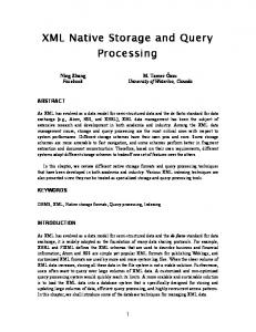
velopment and evaluation of a novel XML Index Selection Tool (XIST) that suggests a suitable set of indices given a combination of an XML schema, a query workload, and data statistics [83]; and (III) the design of an XML micro-benchmark, called the Michigan benchmark, and its use in analyzing the strengths and weaknesses of various XML DBMSs [84]. Another way of viewing the contributions of this thesis is to consider the applicability of the proposed methods to different approaches for managing XML data. There are two extreme approaches in storing and querying XML data. One extreme approach is to use a native XML database whose internal structures map directly onto the hierarchical format of XML data. The other extreme is to use an RDBMS to store and query XML data by mapping XML data to flat relational tables. In the middle of these two extreme approaches are approaches using Object-Oriented Database Management Systems (OODBMSs) and ORDBMSs. The first part of this thesis focuses on storage mapping techniques for managing XML data in an RDBMS and an ORDBMS. The second part of this thesis focuses on the XML index selection, and is applicable to all approaches. The third part of this thesis is the benchmarking effort, which aims to evaluate the strengths and weaknesses of the approaches in the entire range of solutions. In the third part of the thesis, we also present results from running the benchmark on systems at the extreme ends of the spectrum of approaches. Figure 1.1 shows the methods for efficient storage and indexing in XML databases that this thesis focuses on.

1.2

Thesis Outline

This thesis proceeds as follows. Chapter II contains background information on XML, the languages used to describe the structure of XML data, and the languages

III: Benchmarking

Native XML DBMS

I: Storage ObjectOriented DBMS

ObjectRelational DBMS

Relational DBMS

II: XML Index Selection

Figure 1.1: Methods in XML Databases that the Thesis Focuses on used to query XML data. Chapter III presents and evaluates storage techniques that are applicable when the schema of the XML data is known, and Chapter IV considers more general storage techniques used with or without the schema. Chapter V describes the XIST tool which is an index wizard for XML databases that recommends a suitable set of indices to build, given a combination of a workload, a schema, and data statistics. We then describe the Michigan benchmark and present the results from running the benchmark on a number of XML DBMSs in Chapter VI. Conclusions and directions for future work are presented in Chapter VII.

CHAPTER II

Background

This chapter presents basic terminology and background information on XML, XML schema description languages, and XML query languages that are related to this thesis.

2.1

Extensible Markup Language (XML)

In this section, we introduce XML. The small XML document shown in Figure 2.1 will be used as a running example throughout this section.

XML Joe Smith John Jones

Figure 2.1: A Sample XML Document (bib.xml)

9

An XML document consists of the following components: • Elements: Each element represents a logical component of a document. Elements can contain other elements and/or text (character data). The boundary of each element is marked with a start tag and an end tag. A start tag starts with the < character and ends with the > character. An end tag starts with . The root element contains all other elements in the document. In the sample XML document shown in Figure 2.1, the root element of the document is the bib element. Subelements of an element are elements that are directly contained in that element. For example, in the sample document, the article element is a subelement of the bib element. • Attributes: Attributes are descriptive information attached to elements. The values of attributes are set inside the start tag of an element. For example, in Figure 2.1, the expression

sets the value of the attribute id. The main differences between elements and attributes are that attributes cannot contain elements, and there is no “sub-attribute” [50]. In addition, each attribute may be specified only once, and the order of attributes is not important. Further information on XML specification can be found in [14, 35]. In the next section, we briefly present the languages used to describe the structure of XML data.

2.2

XML Schema Description Languages

Several XML Schema languages [10, 11, 13, 41, 72, 73] have been developed, but the two most popular languages are the Document Type Definition (DTD) [10] and

the XML Schema [41]. In this thesis, we use these two languages which are briefly discussed in the following sections. 2.2.1

Document Type Definition (DTD)

A DTD consists of a series of declaration for element types, attributes, entities, etc. It describes what names can be used for element types, where they may occur, and how they fit together. An XML document is valid if its structure conforms to the rules set by its associated DTD. In the remainder of this section, we use the DTD of the sample document, which is shown in Figure 2.2.
bib article article author first last title

(article)*> (title, author+)> id ID #REQUIRED> (first?, last)> (#PCDATA)> (#PCDATA)> (#PCDATA)>

Figure 2.2: A DTD of the Sample XML Document (bib.dtd) A brief overview of the declarations of element types and attributes is given in the following paragraphs. Element Type Declarations: Elements are the foundation of an XML document. Every element in a valid XML document must conform to an element type declared in the DTD. Each Element type declaration must start with the string “ Consider another sample element type declaration:

This rule states that a bib element contains zero or more occurrences of article. If the ∗ in the example were replaced with a +, the bib element would contain one or more occurrences of article. Finally, a ? denotes zero or one occurrence. As another example, consider the following: This element declaration states that an author element contains an optional first element and a required last element. Elements can also contain character data, as shown in this following example: This rule states that the first element does not contain other elements, only text. Attributes Declarations: Attributes are declared for specific element types using an attribute-list declaration. Attributes declarations start with the string “< !ATTLIST”, followed with an element name and a list of attribute declarations. The declaration of an attribute is comprised of its name, its type, and its default value. The general structure of an attributes declaration is below: Consider the following attributes declaration:
article

id

ID

#REQUIRED>

This declaration indicates that the id attribute has the ID type which is used to uniquely identify an element. The default specification of the id attribute is #REQUIRED which denotes that the attribute is required , and its value must be specified by the author of an XML document. That is, in a valid document, every article must have the attribute id. Further information about DTD can be found in [10]. Although DTD has been widely used, it has several limitations. For example, elements and attributes are always of type string and cannot be arbitrarily typed. XML Schema provides a much larger set of data types and a much more powerful method for defining the structure of XML documents. In the next section, we briefly describe XML Schema. 2.2.2

XML Schema

XML Schema is an XML based alternative to DTD for describing the schema of XML documents. As with DTD, XML Schema describes the structure of an XML document. As XML Schema is relatively recent, the schemas of most XML documents are still described using DTD. However, there are several advantages of XML Schema over DTD, such as support for data types and namespaces. Moreover, an XML Schema document is written in XML, thus any XML parser can parse the document. In XML Schema, there are two types of element declarations: the declaration of a simple element and that of a complex element. A simple element contains only text, not any other elements or attributes. The text can be of many different predefined types (boolean, date, integer, etc.), or a user-defined data type. In contrast, a complex element contains other elements and/or attributes and has a complex type which must be defined by a user.



Figure 2.3: An XML Schema of the Sample XML Document (bib.xsd) Elements are declared using the element element, and attributes are declared using the attribute element. Figure 2.3 shows an XML Schema file called “bib.xsd” that declares elements and attributes in the XML document shown in Figure 2.1. Below is the declaration of a simple element in the schema shown in Figure 2.3. In the above element example, the last element has type string, which is a predefined simple type. Below is an example of a complex type definition.

The consequence of this definition is that any element whose type is declared to be authorType (e.g., author in “bib.xml”) must consist of at most one occurrence of first and only one occurrence of last. The occurrence of each element is specified by the minOccurs and maxOccurs attributes, which their default value is one. The sequence element enforces that the first and last elements must appear in a sequence in which first appears before last. Further information about XML Schema can be found in [41]. Once we have languages for describing the XML data and its structure, we need to have a language to query the XML data which is described in the next section.

2.3

XML Query Languages

XQuery [103] is the W3C standard for querying XML data. XQuery is derived from Quilt [20], which in turn borrows features from several other langauges, including XPath [27], XQL [81], and XML-QL [38]. Although XQuery is the most recently proposed XML query language, it uses XPath expressions (and has additional components). XPath is used to specify structural predicate which is the most common type of predicate (and expensive to evaluate) in XML queries. The query workloads that we use in this thesis are specified in XPath since the focus of the thesis is on efficient evaluation of XPath expressions. In this section, we briefly give an overview of XPath.

2.3.1

XPath Expressions

The XPath data model views a document as a tree of nodes. An instance of the XPath language is called an expression. XPath expressions can involve a variety of operations on different kinds of operands. A location path is the most important kind of expressions in the XPath notation. Its syntax is similar to the path expressions used in Unix and Window systems to locate directories and files. A location path has a starting point which is called the context node. The context node can be the root element of the document or other element nodes. A location path selects a set of nodes relative to the context node. A location step has three following parts: • an axis, which specifies the tree relationship between the nodes selected by the location step and the context node. • a node test, which specifies the type of the nodes selected by the location step. • zero or more predicates, which use arbitrary expressions to further refine the set of nodes selected by the location step. The syntax for a location step is the axis name and node test separated by a double colon, followed by zero or more expressions, each in square brackets. For example, in child::para[position()=1], child is the name of the axis, para is the node test, and [position()=1] is the predicate. The node-set selected by the location step is the result from generating an initial node-set from the axis and nodetest, and then filtering that node-set by each predicate in turn. The axis name can be shorthand, and the most important one is that child:: can be omitted from a location step. For example, a location path para[position()=1] is equivalent to child::para[position()=1]. Further information on XPath can be found in [27].

CHAPTER III

Storing and Querying Schema-based XML Documents Using an ORDBMS

3.1

Introduction

As the popularity of the eXtensible Markup Language (XML) [14] continues to grow, large repositories of XML data are likely to emerge. Data management systems for storing and querying these large repositories are urgently needed. Currently, there are two dominating approaches for managing XML repositories [48]. The first approach is to use a native XML database engine for storing and querying XML data sets [90, 91, 98]. This approach has the advantage that it can provide a more natural data model and query language for XML data, which is typically viewed using a tree or graph representation. The second approach is to map the XML data and queries to constructs provided by a Relational Database Management System (RDBMS) [37, 49, 94, 95]. XML data is mapped to relations, and queries on the XML data are converted into SQL queries. The results of the SQL queries are then converted to XML documents before returning the answer to the user. If the mapping of the XML data and queries to relational constructs is automatic, then the user does not need to be involved in the complexity of mapping. One can leverage many decades of research and commercialization efforts by exploiting existing features in an

17

RDBMS. An additional advantage of an RDBMS is that it can be used for querying both XML data and data that exists in the relational systems. The disadvantage of using an RDBMS is that it can lower performance since a mapping from XML data to the relational data may produce a database schema with many relations. Queries on XML data when translated into SQL queries may potentially have many joins, which are expensive to evaluate. In this chapter, we investigate a third approach, namely using an Object-Relational DBMS (ORDBMS) for managing XML data sets. Our motivations for using an ORDBMS are threefold: First, most database vendors today offer universal database products that combine their relational DBMS and ORDBMS offerings into a single product. This implies that the ORDBMS products have all the advantages of an RDBMS. Second, an ORDBMS has a more expressive type system than an RDBMS. Third, an ORDBMS is better suited for storing and querying XML documents that may use a richer set of data types. In using an ORDBMS to store and query XML documents, two aspects that must be considered are how to transform XML data to ORDBMS data and how to transform ORDBMS data back to the original XML data. In this chapter, our focus is on how to transform XML data to ORDBMS data, but not on publishing relational data as XML documents. In addition, we do not focus on issues related to translating XML queries to SQL queries. These issues have been addressed by several works on publishing relational data as XML documents [17,21,46,93] and on translating XML queries to SQL queries [36, 47, 95]. We also do not focus on developing techniques to handle the update of the data since we assume that our techniques are for the more common case of XML applications that are rarely updated, such as dictionaries. We present an algorithm, called XORator (XML to OR Translator), that uses

the Document Type Definitions (DTDs) to map XML documents to tables in an ORDBMS. An important part of this mapping is the assignment of a fragment of an XML document to a new XML data type, called XADT (XML Abstract Data Type). Among several recently proposed XML schema languages, in this chapter, we use DTDs since real XML documents that conform to DTDs are readily available today. Although we focus on using DTD, the XORator algorithm is applicable to any XML schema language that allows defining elements composed of attributes and other nested subelements. In this chapter, we also explore alternative storage organizations for the XADT. Storing a large XML fragment as tagged strings can be inefficient as repeated tags can occupy a large amount of space. To reduce this space overhead, we investigate an alternative compressed storage technique for the XADT. We have implemented the XORator algorithm and the XADT in a leading commercial ORDBMS. In addition, we used real and synthetic data sets to demonstrate the effectiveness of the proposed algorithm. In the experiments, we compare the XORator algorithm with the well-known Hybrid algorithm for mapping XML data to relational databases [94]. Our experiments show that compared to the Hybrid algorithm, the XORator algorithm requires less storage space, has much faster loading times, and in most cases can evaluate queries faster. In many cases, query evaluation using the XORator algorithm is faster by several orders of magnitude, primarily because the XORator algorithm produces a database that is smaller, and results in queries that usually have fewer joins. The remainder of this chapter is organized as follows. We first discuss related work in Section 3.2. Section 3.3 describes the XORator algorithm for mapping XML documents to relations in an ORDBMS using a DTD. We then compare the effec-

tiveness of the XORator algorithm with the Hybrid algorithm in Section 3.4. Finally, we present our conclusions and discuss future work in Section 3.5.

3.2

Related Work

In this section, we discuss and compare previous work on mapping XML data to relational data. Several commercial DBMSs offer some support for storing and querying XML documents [30, 33, 85]. However, these engines do not provide automatic mappings from XML data to relational data, thus the user needs to design an appropriate storage mapping. A number of previous works have been proposed for automatic mapping from XML documents to relations [37, 49, 59, 64, 87, 94, 95]. Deutsch, Fernandez, and Suciu [37] proposed the STORED system for mapping between the semi-structured data model and the relational data model. They adapted a data mining algorithm to identify highly supported patterns for storage in relations. Along the lines of mapping XML data sets to relations, Florescu and Kossmann [49] proposed and evaluated a number of alternative mapping techniques. From their experimental results, the best overall approach is an approach based on separating attribute tables for every attribute name and inlining values into these attribute tables. While these approaches require only an XML instance in the transformation process, Shanmugasundaram et al. [94] used a DTD to find a “good” storage mapping. They proposed three strategies to map a DTD into a relational schema and identified the Hybrid algorithm as being superior to the other ones (in most cases). Most recently, Bohannon et al. [6] introduced a cost-based framework for XML-to-relational storage mapping that automatically found the best mapping for a given configuration of an XML schema, data statistics, and a query workload. Like [6, 94], our proposed XORator algorithm also uses the schema of XML docu-

ments, data statistics, and a query workload to derive a relational schema. However, unlike these previously discussed algorithms, we leverage the data type extensibility feature of an ORDBMS to provide a more efficient mapping. We compare the effectiveness of the XORator algorithm (using an ORDBMS) with the Hybrid algorithm (using an RDBMS) and show that the XORator algorithm generally performs significantly better. Shimura et al. [95] proposed the method that decomposed XML documents into the nodes and stored them in relational tables according to their types. They defined a user data type to store a region of each node within a document. This data type keeps positions of nodes, and its associated methods determine ancestor-descendant and order relationships between elements. Schimdt et al. [87] proposed the Monet XML data model, which is based on the notion of binary associations, and showed that their approach was more efficient than the approach proposed by Shimura et al. [95]. Since the Monet approach uses a mapping scheme that converts each distinct edge in DTD to a table, their mapping scheme produces a large number of tables. For example, using their mapping scheme, the Shakespeare DTD maps to ninety-five tables [87]; on the other hand, using the XORator algorithm, the DTD maps to fifteen tables. Techniques for resolving the data model and schema heterogeneity difference between the relational and XML data models have been examined [60]. The problem of preserving the semantics of the XML data model in the mapping process has also been addressed [65]. These techniques are complementary to the XORator algorithm of the mapping based on the structural information of XML data. Our work is closest to the work proposed by Klettke and Meyer [64]. Both their mapping scheme and the XORator algorithm use a combination of DTD, data

statistics, and a query workload to map XML data to ORDBMS data. However, there is no implementation or experimental evaluation presented in [64]. On the other hand, we implemented the XORator algorithm and compared its performance with that of the Hybrid algorithm. Furthermore, their mapping assumes the existence of the following type constructors: set-of and list-of in an ORDBMS (which are not available in current commercial products). In addition, a user needs to set a threshold to specify which attributes should be assigned to an XML data type; however, there are no guidelines provided in choosing the value of such threshold. In contrast, the XORator algorithm requires only a DTD as a minimum, and it can generate a more efficient mapping with a query workload and data statistics. XORator is a practical demonstration of the use of an XML data type and the advantage of an ORDBMS over an RDBMS. To the best of our knowledge, this work is the first one that presents the implementation of an XML data type and the experimental results on the storage mappings with the XML data type.

3.3

Storing XML Documents in an ORDBMS

In this section, we describe the XORator algorithm for generating an objectrelational schema from a DTD. In our discussions below we will graphically represent a DTD using the DTD graph proposed by Shanmugasundaram et al. [94]. A sample DTD for describing Plays is shown in Figure 3.1, and the corresponding DTD graph is shown in Figure 3.3. Figure 3.1 shows a DTD which states that a PLAY element can have two subelements: INDUCT and ACT in that order. Symbol “?” followed INDUCT indicates that there can be zero or one occurrence of INDUCT subelement nested under each PLAY


PLAY INDUCT ACT SCENE SPEECH PROLOGUE TITLE SUBTITLE SUBHEAD SPEAKER LINE

(INDUCT?, ACT+)> (TITLE, SUBTITLE*, SCENE+)> (TITLE, SUBTITLE*, SCENE+, SPEECH*, PROLOGUE?)> (TITLE, SUBTITLE*, (SPEECH | SUBHEAD)+)> (SPEAKER, LINE)+> (#PCDATA)> (#PCDATA)> (#PCDATA)> (#PCDATA)> (#PCDATA)> (#PCDATA)>

Figure 3.1: A DTD of a Plays Data Set element. Symbol “+” followed ACT indicates that there can be one or more occurrences of ACT subelements nested under each PLAY element. In the INDUCT element declaration, symbol “*” followed SUBTITLE indicates that zero or more occurrences of SUBTITLE subelements are nested under each INDUCT element. A subelement without any followed symbol represents that there must be only one occurrence of that subelement. For example, an ACT element must contain one and only one TITLE subelement. For more details about DTD, please refer to [10]. 3.3.1

Reducing DTD Complexity

The first step in the mapping process is to simplify the DTD information to a form that makes the mapping process easier. We start by applying the set of rules proposed in [94] to simplify the complexity of DTD element specifications. These transformations reduce the number of nested expressions and the number of element items. Examples of these transformations are as follows: • Flattening (to convert a nested definition into a flat representation): (e1 , e2 )∗ → e∗1 , e∗2 When we flatten the nested definition, we may lose some information about the relative orders of the elements. However, this information can be captured

when an XML document instance is loaded into a relation schema by including an attribute that indicates the sibling order of the elements. • Simplification (to reduce multiple unary operators into a single unary operator): ∗ e∗∗ 1 → e1

• Grouping (to group subelements that have the same name): e0 , e∗1 , e∗1 , e2 → e0 , e∗1 , e2 In addition, e+ is transformed to e∗ . The simplified version of the DTD shown in Figure 3.1 is depicted in Figure 3.2.
PLAY INDUCT ACT SCENE SPEECH PROLOGUE TITLE SUBTITLE SUBHEAD SPEAKER LINE

(INDUCT?, ACT*)> (TITLE, SUBTITLE*, SCENE*)> (TITLE, SUBTITLE*, SCENE*, SPEECH*, PROLOGUE?)> (TITLE, SUBTITLE*, SPEECH*, SUBHEAD*)> (SPEAKER*, LINE*)> (#PCDATA)> (#PCDATA)> (#PCDATA)> (#PCDATA)> (#PCDATA)> (#PCDATA)>

Figure 3.2: A DTD of the Plays Data Set (Simplified Version)

3.3.2

Building a DTD Graph

After simplifying the DTD, a DTD graph is built to represent the structure of the DTD. Nodes in the DTD graph are elements, attributes, and operators. The procedure used in the Hybrid algorithm for mapping is based on the assignments of nodes in the DTD graph. After creating the DTD graph, the Hybrid algorithm creates an element graph which expands the relevant parts of the DTD graph into a tree structure. Given an element graph, a relation is created for nodes that satisfy any of these following conditions: 1) the root node of the DTD graph to

access the information which cannot be accessed through other nodes, 2) nodes that are directly below a “*” operator – this corresponds to creating a new relation for a set-valued subelement (the traditional relation system does not support set-valued attributes), and 3) recursive nodes with in-degree greater than one - this corresponds to creating a new relation to handle recursive elements with multiple parents. All remaining nodes (nodes not mapped to a relation) are inlined as attributes under the relation created for their closest ancestor node (in the element graph). We will describe the XORator mapping algorithm in Section 3.3.3. Unlike the DTD graph proposed by Shanmugasundaram et al. [94] where the element with the same name shares the same node, in our DTD graph, the elements that contain characters are duplicated. We choose to do this to make the mapping algorithm more effective and flexible. As an example, consider the the SUBTITLE element which is an element of type PCDATA (contains characters). In the DTD graph [94], the SUBTITLE element appears only once, as shown in Figure 3.3.

We

PLAY

PLAY

?

?

*

* INDUCT

INDUCT

ACT

ACT

* ?

* *

*

*

TITLE

SUBTITLE

PROLOGUE SCENE

? *

*

*

*

SCENE SUBTITLE

PROLOGUE *

TITLE *

* *

*

*

* SPEECH

SPEECH

SUBHEAD

SUBHEAD TITLE

SUBTITLE

* SPEAKER

TITLE

* LINE

Figure 3.3: The DTD Graph for the Plays DTD

SUBTITLE

* SPEAKER

* LINE

Figure 3.4: The Revised DTD Graph for the Plays DTD

choose to decouple the shared SUBTITLE element by rewriting the DTD graph, as shown in Figure 3.4. The advantage of this DTD graph rewriting is that there are two possible choices of the mappings on the SUBTITLE element. The first alternative is to assign the SUBTITLE element as a relation, and the second is to assign each SUBTITLE as an attribute of the relation corresponding to its parent element. On the other hand, using the procedure of the Hybrid algorithm on the DTD graph shown in Figure 3.3, the only available choice for mapping the SUBTITLE element is to assign SUBTITLE as a relation. The advantage of assigning SUBTITLE as an attribute is that fewer joins are required for queries that involve the SUBTITLE element and its parent elements in the DTD graph (such as the INDUCT or the ACT elements). However, the disadvantage of this assignment is that the query which retrieves all SUBTITLE elements must now query all tables that contain data corresponding to the SUBTITLE elements. The decision for the effective mapping depends on the query workload which the XORator algorithm takes into account if it is available. 3.3.3

XORator: Mapping a DTD to an ORDBMS Schema

Unlike the approach of Shanmugasundarum et al. [94], the XORator algorithm does not always assign a node directly below a “*” operator as a relation. XORator allows the mapping on an entire subtree of the DTD graph to an attribute of the XADT type. An XADT attribute can store fragments of an XML document, and its interfaces are described in Section 3.3.4. The implementation details of the XADT in DB2 are described in Section 3.4.1. With XADT, the node below a “*” operator can be assigned as an attribute to store XML fragments. Thus, the number of joins can be reduced when accessing the content of such node. However, inlining large XML fragments can increase the size of the relation, and no query may need to join

nodes in the fragments and their ancestor nodes. The mapping assignment can be more effective by exploiting the availability of a user query workload. The XORator algorithm requires a DTD as a minimal input and accepts a user query workload as an optional input. When the query workload is not available, the XORator algorithm identifies a maximal subgraph such that the root of the subgraph has only one parent node and there is no edge from the node outside the subgraph to any internal node. The XORator algorithm then maps the root of such subgraph to an XADT attribute. When the query workload is available, the XORator algorithm uses a cost-based model to determine whether to assign a node as a relation or as an attribute. The intuition behind the cost-based model is that the elements that are not accessed together should be stored in different relations to reduce the accessing costs of the relations, and the elements that are accessed together should be stored in the same relation to avoid invoking expensive join operations during querying. The algorithm begins with expanding a DTD graph into element trees, and it then assigns the root node of each element tree as a relation. The weights of the remaining nodes are initialized to zero. For each query, the XORator algorithm computes the scan cost of the XML fragment as well as the join cost between the XML fragment and its parent element. The weight of the element is decremented by the join cost and incremented by the scan cost. After examing all queries, the XORator algorithm assigns each node with the non-negative weight to a relation and assigns each node with the negative weight to an attribute. Figures 3.5 and 3.6 describe the XORator algorithm in detail. Let N be the relation containing nodes with the element tag n. The scan cost of table N is estimated proportional to the size of nodes with the element tag n. The

Inputs: A DTD graph, and an optional query workload Output: A relational schema XORator() 1. If a node below a “*” node is accessed by multiple nodes, then 2. Create an element tree with this node as its root node 3. For each element tree ET 4. Assign the root node of the element tree as a relation 5. PostOrderTreeMapping(root(ET)) Figure 3.5: The Overview of the XORator Algorithm equation to estimate the scan cost is described below: scanCost(N ) = ks × size(N ) = ks × card(N ) × avg(tuple(N ))

(3.1)

where ks is the constant, card(N ) is the number of elements matching with node n in XML documents (the number of tuples in table N ), and avg(tuple(N )) is the average number of characters stored inside each node n in XML documents (the average size of a tuple in table N ). For the simplicity of the join cost model, we assume that the database chooses sort merge join as the join operator and creates clustered indices on the primary and foreign keys. Since indices exist on the joined attributes, sorting is simply accomplished by scanning the index. Thus, the sort merge join cost is dominated by the cost for merging sorted tuples that are returned from indices. Let M and N be relations, the join cost equation between M and N is described by the equation below: joinCost(M, N ) = kj × (card(M ) + card(N ))

(3.2)

where kj is the constant, and card(T ) is the cardinality of table T . We note however that the XORator algorithm can be used with other join algorithms, such as nested loop join and hash join by appropriately modeling their costs.

PostOrderTreeMapping(Node n) 1. If (hasChild(n) == true) 2. For each child c 3. PostOrderTreeMapping(c) 4. If (isAssigned(n) == false) 5. w(n) = 0 6. For each query q in query workload Q 7. Let m be the closet ancestor of n (and m has been assigned as a relation) 8. If m ∈ q and n ∈ q 9. Let M be the relation containing m, but not n 10. Let N be the relation containing n 11. Let M N be the relation containing both m and n 12. w(n) = w(n) − joinCost(M, N ) + scanCost(M N ) 13. If query workload is available 14. If w(n) ≥ 0 15. Assign n as a relation 16. Else 17. Assign n as an attribute 18. Else 19. Assign n as an attribute Figure 3.6: The PostOrderTreeMapping Function For the DTD shown in Figure 3.1, the Hybrid algorithm produces the schema which is shown in Figure 3.7. Fields shown in italic are primary keys. As introduced in the mapping algorithms proposed in [94], each relation has an ID field to serve as the primary key, and all relations corresponding to element nodes with a parent have a parentID field to serve as a foreign key to the parent tuple. Moreover, all relations corresponding to element nodes that with multiple parents have a parentCODE field to identify the corresponding parent table. In this work, we add a childOrder field to serve as the order of the element among its siblings. For the DTD shown in Figure 3.1, the XORator algorithm first examines the DTD graph and then marks the root nodes of the element trees. The root node of each element tree, which is highlighted in Figure 3.8, is assigned as a relation. For

play induct

(playID:integer) (inductID:integer, induct parentID:integer, induct title:string) act (actID:integer, act parentID:integer, act childOrder:integer, act title:string, act prologue:string) scene (sceneID:integer, scene parentID:integer, scene childOrder:integer, scene title:string) speech (speechID:integer, speech parentID:integer, speech parentCode:string, speech childOrder:integer) subtitle (subtitleID:integer, subtitle parentID:integer, subtitle parentCode:integer, subtitle childOrder:integer, subtitle value:string) subhead (subheadID:integer, subhead parentID:integer, subhead childOrder:integer, subhead value:string) speaker (speakerID:integer, speaker parentID:integer, speaker childOrder:integer, speaker value:string) line (lineID:integer, line parentID:integer, line childOrder:integer, line value:string) Figure 3.7: The Relational Schema Transformed Using Hybrid each element tree shown in Figure 3.9, it then applies the PostOrderTreeMapping function to decide whether an unassigned node should be a relation or an attribute. As an example to demonstrate the production of the XORator algorithm, consider the following query workload: {scene/speech/line, speech/speaker}. One possible schema generated by the XORator algorithm is shown in Figure 3.10. Note that in contrast to the schema produced using the Hybrid algorithm which is shown in Figure 3.7, the speaker and line elements are assigned as XADT attributes of the speech table instead of being assigned as relations. 3.3.4

Defining an XML Data Type (XADT)

There are two aspects in designing the XADT: choosing a storage format for the data type and defining appropriate functions on the data type. We discuss each of these aspects in turn.

PLAY

Root nodes of element trees

? *

INDUCT ACT

* *

TITLE

? *

SUBTITLE

* PROLOGUE

SCENE * SUBTITLE

TITLE

* *

* SPEECH TITLE

SUBTITLE

SUBHEAD

* * SPEAKER

LINE

Figure 3.8: A DTD Graph When Using XORator

RELATION PLAY

Node to be assigned

INDUCT ACT

* ?

TITLE

* PROLOGUE

SUBTITLE SUBTITLE TITLE SCENE * TITLE

*

SUBTITLE SUBHEAD SPEECH

* SPEAKER

*

LINE

Figure 3.9: Element Trees When Using XORator

play induct

(playID:integer) (inductID:integer, induct parentID:integer, induct title:string) act (actID:integer, act parentID:integer, act childOrder:integer, act title:string, act prologue:string) scene (sceneID:integer, scene parentID:integer, scene childOrder:integer, scene title:string) speech (speechID:integer, speech parentID:integer, speech parentCode:string, speech childOrder:integer speech speaker:XADT, speech line:XADT) subtitle (subtitleID:integer, subtitle parentID:integer, subtitle childOrder:integer, subtitle value:string) subhead (subheadID:integer, subhead parentID:integer, subhead parentCODE:integer, subhead childOrder:integer, subhead value:string) Figure 3.10: The Relational Schema Transformed Using XORator 3.3.4.1

Storage Alternatives for the XADT

A naive storage format is to store in the attribute the text string corresponding to the fragment of the XML document. Since a string may have many repeated element tag names, this storage format may be inefficient. An alternative storage representation is to use a compressed representation for the XML fragment. The approach that we adopt is to use a compression technique inspired by the XMill compressor [67]. The element tags are mapped and replaced by the corresponding integers. A small dictionary is stored in a file to record the mapping between the integers and the element tag names. In some cases where there are few repeated tags in the XADT attribute, the compression does not significantly reduce the storage size but instead incurs additional overhead in compressing and decompressing. Consequently, we have two implementations of the XADT: one that uses compression and the other that does not. The decision to use the “correct” implementation of the XADT is made during the doc-

ument transformation by monitoring the effectiveness of the compression technique. This is achieved by randomly parsing a few sample documents to obtain the storage space sizes in both uncompressed and compressed versions. Compression is used only if the space efficiency is above a certain threshold value. 3.3.4.2

Functions on the XADT

In addition to defining the formats on the XADT, we also define the following functions for accessing and checking the content the XADT attributes: 1. XADT getElm(XADT inXML, VARCHAR rootElm, VARCHAR searchElm, VARCHAR searchKey, INTEGER level): This function examines the XML fragment stored in inXML and returns all rootElm elements that have searchElm within a depth of level from the rootElm. A default value for level indicates that the level information is to be ignored. If searchKey and searchElm are non-empty strings, this function only considers searchElm that contains the searchKey keyword. If only searchKey is an empty string, then the function returns all rootElm elements that have searchElm as subelements. If only searchElm is an empty string, then the function returns all rootElm elements. If both searchElm and searchKey are empty strings, this function returns all rootElm elements in the inXML fragment. The above function answers a short path query with two element tag names, but a long path query can be answered by a composition of multiple calls to this function. This function takes an XADT attribute as input and produces an XADT output which can then be an input to another call of this function. 2. INTEGER findKeyInElm(XADT inXML, VARCHAR searchElm, VARCHAR searchKey):

This function examines all elements with the searchElm tag name in inXML and searches for all searchElm elements that contain the searchKey keyword. As soon as the first searchElm element that contains searchKey is found, the function returns a value of 1 (true). Otherwise, the function returns a value of 0 (false). If only searchKey is an empty string, this function simply checks whether inXML contains any searchElm element. If only searchElm is an empty string, this function simply checks whether searchKey is part of the content of any element in inXML. Both searchElm and searchKey cannot be empty strings at the same time. This function is a special case of the getElm function defined above and is implemented for efficiency purposes only. 3. XADT getElmIndex(XADT inXML, VARCHAR parentElm, VARCHAR childElm, INTEGER startPos, INTEGER endPos): This function returns all childElm elements that are children of the parentElm elements and that with the sibling order from the startPos to endPos positions. If only parentElm is an empty string, then childElm is treated as the root element in the XADT. Note that childElm cannot be an empty string. More specialized functions can be implemented to further improve the performance using the XADT. Sample queries for both algorithms posed on a data set describing Shakespeare Play are depicted in Figures 3.11 and 3.12.

Figure 3.11 shows query QE1, which

retrieves the lines that are spoken by the speaker HAMLET in the act speeches, and the lines contain the keyword “friend”. Figure 3.11(a) shows the uses of the XADT functions: getElm and findKeyInElm. Figure 3.11(b) shows query QE1 executed

over the database produced by the Hybrid algorithm. SELECT FROM WHERE AND AND AND

getElm(speech line, ‘LINE’, ‘LINE’, ‘friend’) speech, act findKeyInElm(speech speaker, ‘SPEAKER’, ‘HAMLET’) = 1 findKeyInElm(speech line, ‘LINE’, ‘friend’) = 1 speech parentID = act ID speech parentCODE = ‘ACT’ (a) Using the XORator Algorithm

SELECT FROM WHERE AND AND AND AND AND

line val speech, act, speaker, line speech parentID = act ID speech parentCODE = ‘ACT’ speaker parentID = speech ID speaker val = ‘HAMLET’ line parentID = speech ID line val like ‘%friend%’

(b) Using the Hybrid Algorithm

Figure 3.11: Query QE1 in Both Algorithms Figure 3.12 shows query QE2, which returns the second line in each speech. Figure 3.12(a) shows the uses of the getElmIndex function, and Figure 3.12(b) shows query QE2 executed over the database produced by the Hybrid algorithm.

SELECT FROM

getElmIndex(speech line, ‘’,‘LINE’,2,2) speech (a) Using the XORator Algorithm

SELECT FROM WHERE AND

line val speech, line line parentID = speech ID line childOrder = 2

(b) Using the Hybrid Algorithm

Figure 3.12: Query QE2 in Both Algorithms

3.3.5

An Unnest Operator

In addition to the functions described above, we also need an unnest operator to unnest elements stored in an XADT attribute. As described in Section 3.3.3, using the XORator algorithm, it is possible to map an entire subtree of a DTD graph below a “*” node to an XADT attribute. One can then view the XADT attribute as a set of XML fragments. When a user needs to examine individual elements in the set of XML fragments, an unnest operator is required. For example, for the Plays DTD (of Figure 3.1), consider the query that requests distinct speakers. Using XORator, speakers are stored as an XADT attribute. It is possible that one speech has many speakers. Thus, the speaker attribute, which is of type XADT, can contain the XML fragment s1s2. On the other hand, another XML fragment may contain only one speaker, s1. To retrieve distinct speakers, we need to unnest the speakers in each XML fragment. In our implementation, we define an unnest operation using a table User-Defined Function (UDF). A table UDF is an external UDF which delivers a table to the SQL query in which it is invoked in the FROM clause. Figure 3.13 shows the content of table speakers before we unnest the speaker attribute and the result of the query that unnests the speaker attribute. The first parameter (speaker) of table unnest is the attribute containing nested elements. The second parameter of this function, speaker, is the tag name of elements to be unnested. unnestedS is the table that is returned from function unnest. This table has one attribute, out, which contains unnested elements.

QUERY: SELECT FROM

speaker speakers

RESULT: SPEAKER ————————————————————— s1s2 s1 2 record(s) selected. (a) Before Unnesting

QUERY: SELECT FROM

DISTINCT unnestedS.out as SPEAKER speakers, table(unnest(speaker, ‘speaker’)) unnestedS

RESULT: SPEAKER ————————————————————— s1 s2 2 record(s) selected. (b) After Unnesting

Figure 3.13: Before and After Unnesting the speaker Attribute

3.4

Performance Evaluation

In this section, we present the results of implementing the XORator algorithm (along with the XADT) and compare its effectiveness with the Hybrid algorithm [94]. We evaluated the effectiveness of the two algorithms using both real and synthetic data sets. The real data set is the well-known Shakespeare plays data set [8]. The synthetic data set uses an XML document generator [29] to generate data conforming to the SIGMOD Proceedings DTD [79]. In Section 3.4.3, we present the experimental results comparing the Hybrid and the XORator algorithms using the Shakespeare plays data set. We also tested the XORator algorithm using a data set that is “deep” and “narrow”. In such data set, the XORator algorithm may map large XML fragments to XADT attributes. This type of data set allows us to test how effective the XORator algorithm is when most of the data may be inside the XADT attribute. We used the SIGMOD Proceedings data set for this purpose. The results of the experiment with this DTD are presented in Section 3.4.4. 3.4.1

Implementation Overview

We implemented the XADT in a leading commercial ORDBMS. Two versions of the XADT were implemented based on the two storage alternatives discussed in Section 3.3.4.1. The first implementation stores all element tag names as strings. The second stores all the element tag names as integers and uses a dictionary to encode the tag names as integers, thereby storing the XML data in a compressed format. In both cases, the XADT was implemented on top of the VARCHAR data type provided by the ORDBMS. We used the C string functions to implement the functions outlined in Section 3.3.4.2.

To parse the XML documents, we used the IBM’s Alphawork Java XML Parser (XML4J V.2.0.15) [28]. We modified the parser so that it read the DTD and applied the XORator and the Hybrid algorithms, generating SQL commands to create tables in the database. The modified parser also chooses the storage alternative. The compressed format is chosen only if it reduces the storage space by at least 10%. In our current implementation, all tuples in a table with an attribute of type XADT use the same storage representation. To determine which storage alternative to use, we randomly parse a few sample documents to obtain the storage space sizes in both uncompressed and compressed cases. 3.4.2

Experimental Platform and Methodology

We performed all experiments on a single-processor 1.2 GHz Pentium Celeron machine running Windows XP with 256 MB of main memory. The buffer pool size of the database was set to 32 MB. All the UDFs on the XADT were run in a NOT FENCED mode in the database. We choose the NOT FENCED mode because the FENCED option causes the UDF run outside the database address space, and this incurs a significant performance penalty. Before executing queries, we collected statistics and created indices as suggested by the index selection tool of the database. The execution times reported in this section are cold numbers. Each query was run five times, and the average of the middle three execution times was reported. 3.4.3

Experiments Using the Shakespeare Plays Data Set

In this experiment, we loaded the Shakespeare play documents into the database using the two mapping algorithms. The DTD corresponding to the Shakespeare

Plays data set [8] is shown in Figure 3.14.


(TITLE,FM,PERSONAE,SCNDESCR, PLAYSUBT,INDUCT?, PROLOGUE?,ACT+,EPILOGUE?)>

Figure 3.14: The DTD of the Shakespeare Data Set For this data set, the XORator algorithm chooses the uncompressed storage alternative since the compressed representation reduces the storage space less than 10%. The schemas for these relations are presented in Appendix A.1. To produce a large data set, we made eight copies of the the original Shakespeare data set (8 MB), thus the total size of the data set is 64 MB. To assess the scalability of both algorithms, we loaded the text files to the database two and four times. We refer to these configurations as DSx2 and DSx4 respectively, and we refer to the original configuration as DSx1. Table 3.1 shows the comparisons of the number of tables, the database sizes, and the index sizes of the two algorithms. As shown in the table, the size of the database produced by XORator is approximately 60% of that produced by Hybrid, and the index size produced by XORator is approximately 5% of that produced by Hybrid.

The database and the index sizes of XORator are much smaller than those of Hybrid because XORator produces a mapping with fewer tables and smaller tuple sizes. Hybrid XORator Number of tables

17

15

Database size (MB)

119

72

Index size (MB)

282

13

Table 3.1: Database Statistics for the Shakespeare DSx1 Data Set The query set used in this experiment is described below: QS1. Selection: Retrieve the lines that have the keyword “Rising” in the text of the stage direction. QS2. Simple path expression: Retrieve the lines that have stage directions associated with the lines. QS3. Flattening: In each speech, list the speakers and the lines that they speak. QS4. Multiple selections on a single path: In the play “Romeo and Juliet”, retrieve the speeches that are spoken by the speaker “Romeo” and that the speech lines contain the keyword “love.” QS6. Order access: Retrieve the second line of all speeches that are in prologues. We choose this simple set of queries because it allows us to study the core performance issues and is an indicator of performance for more complex queries. In this work, we do not focus on automatically rewriting XML queries into equivalent SQL queries. We refer the reader to proposed query rewriting algorithms from XML query languages to SQL [19, 95, 107]. The SQL statements corresponding to the above queries for both algorithms are presented in Appendix A.2. The result of executing queries QS1 through QS6, the data loading times, and the transformation times for the Shakespeare DSx1 data set are shown in Table 3.2.

Query

Execution Times (seconds) Hybrid XORator QS1 17.68 4.08 QS2 32.01 4.37 QS3 29.01 7.61 QS4 7.14 0.23 QS5 20.32 0.25 QS6 5.04 0.04 Loading 3029.00 196.00 Transformation 298.00 475.00 Table 3.2: Execution Times of Hybrid and XORator for the Shakespeare DSx1 Data Set

The transformation time includes time taken for parsing the documents, mapping a DTD to a relational schema, and writing the files to be loaded to the database. The transformation time of Hybrid is less than that of XORator because XORator spends time on collecting data statistics and computing a cost-based mapping using a given workload. We provide a graphical representation to emphasize the performance difference between the two algorithms in Figure 3.15. This figure illustrates the ratios of the execution times using Hybrid and XORator on a log scale. Since the size of the database produced using XORator is about 60% of that produced using Hybrid, XORator results in smaller loading times. The XORator algorithm also results in significantly smaller execution times for all queries. In most queries, the XORator algorithm is several orders of magnitude faster than the Hybrid algorithm. This is because all queries using XORator requested at least one fewer join than the corresponding query using Hybrid. As the data size increases, the optimizer sometimes chooses different query plans for the same query. Thus, for some queries, such as query QS1, the ratio of the performance of Hybrid and XORator changes inconsistently with respect to the database size. In some queries, such as query QS3, the XORator algorithm consistently scales

Hybrid/XORator Performance Ratios (log scale)

1000 108.4 81.3 44.4

100 31.0

10

4.3 4.0 5.2

7.4 3.5

5.0

43.4

3.8 4.3 4.8

DSx1 DSx2 DSx4

126

27.6 15.5

37.8

5.8

4.1

3.3

1 0.1 0.01 0.001

QS1

QS2

QS3

QS4

QS5

QS6

Loading

Figure 3.15: Hybrid/XORator Performance Ratios on a Log Scale as Database Sizes Increase for the Shakespeare Data Sets

better than the Hybrid algorithm. In query QS3, the Hybrid algorithm requests external sorting as the data size is larger than the buffer pool size. On the other hand, in query QS6, Hybrid consistently scales better than XORator because XORator requests additional sorting as the data size becomes larger than the buffer pool size. We also compare the mapping generated by the XORator algorithm with the extreme types of grouping: minimal grouping (assigning every element as a relation) and maximal grouping (assigning only shared nodes with multiple occurrences as relations). Figure 3.16 shows the performance of the mapping generated by the XORator algorithm, the minimal grouping, and the maximal grouping on the Shakespeare DSx1 data set.

As shown in Figure 3.16, the performance of the minimal

grouping is much worse than that of the maximal grouping due to a large number of relations and multiple requested join operations. Thus, for the Shakespeare DSx2 and DSx4 data sets, only the maximal grouping and the mapping produced by XORator are compared in Figures 3.17 and 3.18. As shown in these figures, the performance

Execution Times (seconds) (log scale)

Minimal grouping 1000

Maximal grouping XORator

100 17.7

10

28.0

120

196

28.9 15.1 7.7 7.6

4.1 4.1

2920

4.5 4.4

6.4

5.1

1 0.2 0.2

0.3 0.3

0.1

0.1 0.04

0.01

QS1

QS2

QS3

QS4

QS5

QS6

Loading

Figure 3.16: Performance of Different Mappings for the Shakespeare DSx1 Data Set

of the mapping generated by XORator is usually higher than or at least the same as that of the maximal grouping. However, the loading times of the maximal grouping are less than those of XORator since the maximal grouping results in the schema with fewer relations. 3.4.4

Experiments Using the SIGMOD Proceedings Data Set

This section presents the experimental results when using the SIGMOD Proceedings data set. The DTD of this data set is an example of a deep DTD. With such DTD, the XORator technique may map large fragments of XML data to the XADT attributes. This DTD is a representative of the worst-case scenario for the XORator algorithm since almost an entire document can be mapped to an XADT attribute. The DTD corresponding to the SIGMOD Proceedings data set has seven levels. Elements that are likely to be queried often, such as “author”, are at the bottom-most level. The DTD is depicted in Figure 3.19. The schemas of these relations are in Appendix A.3.

Execution Times (seconds) (log scale)

Maximal grouping XORator

260

390

100 23.9 23.7

24.5 24.5

28.6 28.3

10 2.7

1

1.8 1.6 0.5

0.5 0.5

0.1 0.01

QS1

QS2

QS3

QS4

QS5

QS6

Loading

Figure 3.17: Performance of Different Mappings for the Shakespeare DSx2 Data Set

Execution Times (seconds) (log scale)

1000 100

Maximal grouping XORator 43.8 38.5

42.2 37.4

518

773

57.2 54.2

10

6.8 6.5

5.9 5.1 1.0 1.0

1 0.1 0.01

QS1

QS2

QS3

QS4

QS5

QS6

Loading

Figure 3.18: Performance of Different Mappings for the Shakespeare DSx4 Data Set


(volume,number,month,year,conference, date,confyear,location,sList)> volume (#PCDATA)> number (#PCDATA)> month (#PCDATA)> year (#PCDATA)> conference (#PCDATA)> date (#PCDATA)> confyear (#PCDATA)> location (#PCDATA)> sList (sListTuple)*> sListTuple (sectionName,articles)> sectionName (#PCDATA)> sectionName SectionPosition CDATA #IMPLIED > articles (aTuple)*> aTuple (title,authors,initPage,endPage, Toindex,fullText)> title (#PCDATA)> title articleCode CDATA #IMPLIED> authors (author)*> author (#PCDATA)> author AuthorPosition CDATA #IMPLIED > initPage (#PCDATA)> endPage (#PCDATA)> Toindex (index)?> index (#PCDATA)> Toindex %Xlink;> fullText (size)?> size (#PCDATA)> fullText %Xlink;>

Figure 3.19: The DTD of the SIGMOD Proceedings Data Set For this data set, the XORator algorithm chooses to use the compressed storage alternative since the compressed representation reduces database size by approximately 13%. To produce large data sets, we took the original generated SIGMOD Proceedings data set and loaded it multiple times, producing data sets with configurations: DSx1, DSx2, and DSx4. The total input size of the SIGMOD Proceedings DSx1 data set is 64 MB. Table 3.3 shows the comparisons of the number of tables,

database sizes, and the index sizes of the two algorithms for the SIGMOD Proceedings DSx1 data set. Hybrid XORator Number of tables

7

6

Database size (MB)

89

67

Index size (MB)

86

39

Table 3.3: Database Statistics for the SIGMOD Proceedings DSx1 Data Set The query set in this experiment is described below: QG1. Selection: Retrieve the authors of the papers with the keyword “title 1” in the paper title. QG2. Simple path expression: List all authors and their paper titles. QG3. Flattening: Retrieve the proceeding section names of each conference. QG4. Multiple selections on a single path: Retrieve the first page of the paper that is in section “section1” and that is written by author “author1”. QG5. Multiple selections on multiple paths: Retrieve the first page of the paper with the title containing the keyword “title 1” and that is written by “author 2”. QG6. Order access: Retrieve the second author of the papers with the keyword “title2” in the paper title. The SQL statements corresponding to the above queries for both algorithms are presented in Appendix A.4. The result of executing queries QG1 through QG6, the data loading times, and the transformation times for the SIGMOD Processong DSx1 data set are shown in Table 3.4. The transformation time of XORator is longer than that of Hybrid because of the computation time in finding an appropriate mapping and compressing data. To

Query

Exec. Times (seconds) Hybrid XORator QG1 8.62 5.38 QG2 8.01 3.77 QG3 1.83 1.87 QG4 0.84 1.42 QG5 8.87 4.60 QG6 5.26 0.35 Loading 1009.00 507.00 Transformation 869.00 1445.00 Table 3.4: Execution Times of Hybrid and XORator for the SIGMOD Proceedings DSx1 Data Set

emphasize the performance difference between Hybrid and XORator for the various data sets, we provide a graphical representation of the ratios of the execution times

Hybrid/XORator Performance Ratios (log scale)

of queries using Hybrid over those of using XORator in Figure 3.20. 100

DSx1 DSx2 DSx4

14.9

10 1.6

1

2.1 1.0 1.3

1.7 1.0

1.0 1.1 1.1

1.1

1.5

1.7

2.6 1.5

1.5

1.9

2.0 2.1 2.1

0.6

0.1

0.01

QG1

QG2

QG3

QG4

QG5

QG6

Loading

Figure 3.20: Hybrid/XORator Performance Ratios on a Log Scale as Database Sizes Increase for the SIGMOD Proceedings Data Sets

As shown in Figure 3.20, the execution times of queries when using XORator are usually smaller than those when using Hybrid except for query QG4 on the DSx1

data set. In most of queries, the XORator algorithm outperforms Hybrid because XORator requests fewer joins. However, in query QG4, the predicates are highly selective, and thus the join cost between the indexed tuples is low when using the Hybrid algorithm. On the other hand, when using XORator, the scan cost of the XADT attribute is requested. The scan cost is relatively higher than the join cost when using Hybrid. However, as the database size increases, in query QG4, the scan cost grows relatively slower than the join cost. Thus, in query QG4 on the DSx2 and DSx4 data sets, the XORator outperforms the Hybrid algorithm. We also compared the mapping generated by the XORator algorithm with the extreme types of mappings: minimal and maximal groupings. Figure 3.21 shows that the mapping produced by XORatoroutperforms the minimal and maximal groupings in all queries, except when loading the data. The loading times of the maximal grouping are much less than those of the XORator mapping and the minimal grouping because the maximal grouping generates the schema with only one relation which has a large XADT attribute. To test the effectiveness of data compression, we loaded the SIGMOD Proceedings data set using both the uncompressed and compressed storage alternatives. The performance comparison between the uncompressed and compressed storage is depicted in Figure 3.22. The compressed XADT outperforms the uncompressed XADT for most queries. However, for a few queries, such as query QG3, the performance of the uncompressed and compressed XADT is equivalent because the queries do not access any XADT attribute. We also ran the experiments on the compressed Shakespeare data set and found out that the compression has only a very small effect on the query performance.

Execution Times (seconds) (log scale)

2302

Minimal grouping Maximal grouping XORator 100 10

11.815.4

9.5 5.4

35

36.3

24.1

17.1

9.7 8.0

507

10.4 4.8 4.6

3.8 1.9

1.5 1.4

1.5

1 0.4

0.1 0.01

QG1

QG2

QG3

QG4

QG5

QG6

Loading

Figure 3.21: Performance of Different Mappings for the SIGMOD Proceedings DSx1 Data Set

XORator: Uncompressed XORator: Compressed

527 507

Time (seconds) (log scale)

100 10

6.2 5.4

4.6 3.8

5.4 4.6 1.9 1.9

2.1

1.4

1

0.4 0.4

0.1 0.01

QG1

QG2

QG3

QG4

QG5

QG6

Loading

Figure 3.22: Performance of Uncompressed and Compressed Versions for the SIGMOD Proceedings DSx1 Data Set

3.5

Conclusion and Future Work

We have proposed and evaluated XORator, an algorithm for mapping XML documents with DTDs to relations in an ORDBMS. Using the data type extensibility mechanisms provided by an ORDBMS, we added a new data type called XADT that can store and query arbitrary fragments of an XML document. The XORator algorithm maps a DTD to an object-relational schema that may have attributes of type XADT. Using an implementation in a leading commercial ORDBMS, we show that the XORator algorithm generally outperforms the well-known Hybrid algorithm that is used for mapping XML documents to relations in an RDBMS. The primary reason for this superior performance is that queries in the XORator algorithm usually execute fewer joins. For future work, we are interested in expanding the mapping rules to accommodate additional factors, such as the selectivities of predicate values. More accurate cost models for the chosen join algorithms can also further enhance the quality of schemas produced by XORator.

CHAPTER IV

Storing and Querying XML Documents Using a Relational Database

4.1

Introduction

In the previous chapter, we proposed the XORator algorithm for mapping XML documents with XML schemas to relations. However, in some cases, XML documents exist without any associated schema information, thus the XORator algorithm is not applicable for such documents. A number of different approaches have been proposed to map XML data to relations, independent of XML schemas [49, 95, 107, 108]. However, no approach has been shown to be consistently superior to other methods. Moreover, there is no systematic evaluation of the strengths and weaknesses of each approach. In this chapter, we propose a mapping scheme which outperforms other approaches for most queries. Furthermore, we identify the types of queries for which each approach is suitable. Since this mapping scheme can be applied on both schema-based and schema-less XML documents, it is not alternative to the XORator technique. It is rather complementary to the XORator technique. To efficiently evaluate XML queries, it is important to quickly determine the structural relationships among any pair of nodes. Structural relationships can be determined by associating each node with a numbering scheme. One of the most

52

popular method is Dietz’s numbering scheme [40], which has been adopted by several XML query evaluation techniques [3, 54, 66, 108]. In this numbering scheme, a document is modeled as a tree. Each tree node is assigned three numbers: the node’s preorder and postorder ranks, and the node’s level. In a preorder (postorder) traversal, a node is visited and assigned its preorder (postorder) rank before (after) its children are recursively assigned from left to right. If the document is read sequentially, elements are accessed in the same order as their preorder ranks. Using Dietz’s numbering scheme, the following properties hold: • Node v is an ancestor of node u iff (i) preorder(v) < preorder(u), and (ii) postorder(u) < postorder(v). • Node v is a parent of node u iff (i) preorder(v) < preorder(u), (ii) postorder(u) < postorder(v), and (iii) level(v) = level(u) − 1 To evaluate path expressions in a relational system, there are two dominating approaches. The first is to use primary-foreign keys of relations to establish a parentchild relationship between elements [49,94]. The other approach is to use the element positions in XML documents (preorder, postorder, level) [95,107,108]. The advantage of the primary-foreign keys approach is that the queries containing only parent-child relationships are evaluated very quickly since there are indices built on the primaryforeign keys. However, the disadvantage of this approach is the poor performance of ancestor-descendant queries. When using the primary-foreign keys approach to evaluate ancestor-descendant queries, the number of join operations can be as many as the number of steps of the longest path in the document tree [107]. On the other hand, using node positions, only direct joins between the ancestors and descendants are needed. Another problem of the primary-foreign keys approach is that recursive

SQL statements are required to answer ancestor-descendant queries which tend to be very expensive to evaluate [84]. We improve existing node position schemes by encoding extra information about the node’s parent and including the node’s path information. Our experimental results show that this additional information can dramatically reduce query response times in relational systems. In addition, we identify types of queries on which each approach performs well. This identification and the query workload information are useful in determining which node information to keep for storing and querying XML data more efficiently in relational systems. Although we did not perform the experiments on a native XML database, the techniques presented in this chapter can be applied in such database. The remainder of this chapter is organized as follows. We first discuss different mapping approaches in Section 4.2. We then evaluate and compare the effectiveness of these mapping approaches in Section 4.3. Related work is discussed in Section 4.4. Finally, we present our conclusions and discuss future work in Section 4.5.

4.2

Different Mapping Approaches

In this section, we present three different mapping approaches. All of these approaches model a document as a tree and use the word positions of elements to establish the structural relationships between elements. When presenting these approaches, we use the sample XML document in Figure 4.1 as an input document. We first present the relational schemas and sample SQL queries of the approach which we refer to as Begin-End-Level (BEL) [108] and those of the approach which we refer to as Begin-End-Level-Path (BELP) [95]. We then present our proposed mapping approach which we refer to as BEL+Parent-ID (PAID).

1 2 3 Act One 7 8 Scene One 12 13 Romeo 16 Hello, Juliet 20 21 22 Juliet 25 Good morning, Romeo 30 31 32 33

Figure 4.1: A Sample XML Document (with Word Positions in Bold)

4.2.1

The Begin-End-Level (BEL) Approach

In the Begin-End-Level (BEL) approach [108], containment queries are processed using inverted lists. Each inverted list records the occurrences of a word or an element which is referred to as “term”. Each occurrence is indexed by its document number (docno), its word position (begin:end), and its nesting depth within the document (level). The positions of elements and words (begin, end, wordno) are generated by counting word numbers in an input XML document. The occurrence of an element is denoted as (docno, begin:end, level), and the occurrence of a text word is denoted as (docno, wordno, level). Elements and text words are stored in the Element and Text relations, respectively. The storage of attributes is not discussed in [108]. To handle documents that have attributes, one can extend this approach by treating an attribute like an element and append attribute information in Element. However, from our experimental results, separately storing attribute information in the Attribute relation results in superior performance. Note that we add the order attribute in the Element relation to answer the queries with order predicates. The schemas of the three relations (Element, Text, and Attribute) are as following: • Element: This relation stores the information associated with each element node. This information includes element tag, document identifier, element order, and element position (begin, end, level). The schema of this relation is Element(term string, docID integer, order integer, begin integer, end integer, level integer). • Text: This relation stores the information associated with text contained in each element node. This information includes a text word, document identifier, and text position (wordno, level). The schema of this relation is

Text(term string, docID integer, wordno integer, level integer). • Attribute: This relation stores the information associated with each attribute node. This information includes attribute name, attribute value, document identifier, and attribute position (begin, end, level). The schema of this relation is Attribute(term string, value string, docID integer, begin integer, end integer, level integer). Using this approach, the content of the relations storing sample XML data in Figure 4.1 is shown in Figures 4.2-4.3. The corresponding SQL query for the path expression SPEECH/SPEAKER is shown in Figure 4.4. term docID order begin end level PLAY 1 1 1 33 1 ACT 1 1 2 32 2 TITLE 1 1 3 6 3 SCENE 1 1 7 31 3 TITLE 1 1 8 11 4 SPEECH 1 1 12 20 4 SPEAKER 1 1 13 15 5 LINE 1 1 16 19 5 SPEAKER 1 1 22 24 5 SPEECH 1 2 21 30 4 LINE 1 1 25 29 5 Figure 4.2: The Element Relation of BEL

4.2.2

The Begin-End-Level-Path (BELP) Approach

In [95, 107], the Begin-End-Level-Path (BELP) approach decomposes an XML document into nodes on the basis of its tree structures. A relation is created for each node type, and a path relation stores path information from the root node to each

term docID wordno level Act 1 4 4 One 1 5 4 Scene 1 9 5 One 1 10 5 Romeo 1 14 6 Hello 1 17 6 Juliet 1 18 6 Juliet 1 23 6 Good 1 26 6 morning 1 27 6 Romeo 1 28 6 Figure 4.3: The Text Relation of BEL

select from where and and and and and

espeaker.docID, espeaker.begin element espeaker, element espeech espeech.term = ‘SPEECH’ espeaker.term = ‘SPEAKER’ espeech.begin < espeaker.begin espeaker.end < espeech.end espeech.level = espeaker.level - 1 espeech.docID = espeaker.docID

Figure 4.4: A SQL Query When Using BEL

of other nodes. Nodes of different XML documents are stored in the same relation as long as they are of the same type. In the original BELP approach [95], the position of the node has the REGION type (User Abstract Data Type) [95]. We do not store the position within the REGION type because our experimental results indicate that it is more effective to store the begin and end positions as attributes on which the B+ tree indices can be built. Traditional RDBMSs do not allow the users to build indices on a user-defined type, such as REGION. Although the level information is not originally included [95], we include it to distinguish between the parent-child and the ancestor-descendant relationships. In the BELP approach, each word occurrence is assigned an integer corresponding to its position within the document, and each tag is assigned a real number. The integer part of the real number indicates the position number of the preceding word. The decimal part indicates the position of the tag in the current depth-first traversal. When visiting the root node or the node visited immediately following the text word, the decimal part is initialized to one. When visiting the other nodes, the decimal part is incremented. The position of the element is assigned a real number to minimize the effects of the appearances of the element tags on a word-based proximity search on element content [95]. Figure 4.5 shows the data graph with the assignment of the region of each node in the XML data of Figure 4.1. The details of the schemas of the Element, Attribute, Text, and Path relations are as follows: • Element: This relation stores the information associated with each element node. This information includes document identifier, path identifier, occurrence order, and element position. The schema of this relation is

/PLAY (0.01,11.05)

ACT (0.02,11.04)

TITLE (0.03,2.01)

SCENE (2.02,11.03)

Act One (1,2) TITLE (2.03, 4.01)

SPEECH (4.02,7.02)

Scene One (3,4) SPEAKER (4.03, 5.01)

SPEECH (7.03,11.02)

SPEAKER (7.04, 8.01) LINE (5.02,7.01)

Juliet (8,8)

Romeo (5,5)

LINE (8.02,11.01)

Good morning, Romeo (9,11)

Hello, Juliet (6,7)

Figure 4.5: The Tree Structure in the Sample Document When Using BELP

Element(docID integer, pathID integer, order integer, begin double, end double, level integer). • Attribute: This relation stores the information associated with each attribute node. This information includes document identifier, path identifier, attribute value, and attribute position. The schema of this relation is Attribute(docID integer, pathID integer, attvalue string, begin double, end double, level integer). • Text: This relation stores the information associated with the content of each element node. This information includes document identifier, path identifier, text value, and text position. The schema of this relation is Text(docID integer, pathID integer, value string, begin double, end double, level integer). • Path: This relation stores the information about the path expression starting from the root node. This information includes path expression and path identifier. The schema of this relation is Path(pathExp string, pathID integer). Using this approach, the content of the relations storing sample XML data in Figure 4.1 is shown in Figures 4.6-4.8. The corresponding SQL query for the path expression SPEECH/SPEAKER is shown in Figure 4.9. 4.2.3

The Parent-ID (PAID) Approach

The Parent-ID (PAID) approach is an extension of the Begin-End-Level (BEL) approach. In addition to using (begin, end, level) in solving containment relationship queries, we use the IDs of the parent nodes to quickly determine elements that have

docID pathID order begin end level 1 0 1 0.01 11.05 1 1 1 1 0.02 11.04 2 1 2 1 0.03 2.01 3 1 3 1 2.02 11.03 3 1 2 1 2.03 4.01 4 1 5 1 4.02 7.02 4 1 6 1 4.03 5.01 5 1 7 1 5.02 7.01 5 1 5 2 7.03 11.02 4 1 6 1 7.04 8.01 5 1 7 1 8.02 11.01 5 Figure 4.6: The Element Relation of BELP docID pathID value begin end level 1 2 Act One 1 2 4 1 4 Scene One 3 4 5 1 6 Romeo 5 5 6 1 7 Hello, Juliet 6 7 6 1 6 Juliet 8 8 6 1 7 Good morning, Romeo 9 11 6 Figure 4.7: The Text Relation of BELP parent-child relationship, and use the path information to quickly retrieve elements that match a given path. The schemas of the relations in this approach are as follows: • Element: This relation stores data associated with each element node. This information includes document identifier, element tag name, path identifier, element order, element position, and parent identifier. The relational schema is Element(docID integer, term integer, pathID integer, order integer, begin integer, end integer, level integer, parentID integer). • Path: This relation provides the mapping between path name and path identifier. The relational schema is

pathExp /PLAY /PLAY/ACT /PLAY/ACT/TITLE /PLAY/ACT/SCENE /PLAY/ACT/SCENE/TITLE /PLAY/ACT/SCENE/SPEECH /PLAY/ACT/SCENE/SPEECH/SPEAKER /PLAY/ACT/SCENE/SPEECH/LINE

pathID 0 1 2 3 4 5 6 7

Figure 4.8: The Path Relation of BELP select from

espeaker.docID, element espeaker, element espeech, where pspeaker.pathExp and pspeaker.pathID and pspeech.pathExp and pspeech.pathID and espeech.begin and espeaker.end and espeech.level and espeech.docID

espeaker.begin path pspeaker, path pspeech like ‘%SPEECH/SPEAKER’ = espeaker.pathID like ‘%SPEECH’ = espeech.pathID < espeaker.begin < espeech.end = espeaker.level - 1 = espeaker.docID

Figure 4.9: A SQL Query When Using BELP Path(pathExp string, pathID integer). • Attribute: This relation stores data associated with each attribute node. This information includes attribute name identifier, document identifier, attribute value, attribute identifier, and the identifier of the element that contains the attribute. The relational schema is Attribute(attrName string, docID integer, begin integer, attrValue string, level integer, parentID integer). • Text: This relation stores data associated with text contained in each element node. This information includes the text value, document identifier, the po-

sition of the word in the text, the identifier of the element that contains the word. The relational schema is Text(term string, docID integer, wordno integer,

level integer,

parentID integer). Using this approach, the content of the relations storing the sample XML data shown in Figure 4.1 is depicted in Figures 4.10-4.12. With the attribute parentID, one can evaluating path expression SPEECH/SPEAKER using SQL statements as shown in Figures 4.13-4.14. docID term pathID order begin end level parentID 1 TITLE 2 3 6 1 3 2 1 TITLE 4 8 11 1 4 7 1 SPEAKER 6 13 15 1 5 12 1 LINE 7 16 19 1 5 12 1 SPEECH 5 12 20 1 4 7 1 SPEAKER 6 22 24 1 5 21 1 LINE 7 25 29 1 5 21 1 SPEECH 5 21 30 2 4 7 1 SCENE 3 7 31 1 3 2 1 ACT 1 2 32 1 2 1 1 PLAY 0 1 33 -1 1 -1 Figure 4.10: The Element Relation of PAID pathExp /PLAY /PLAY/ACT /PLAY/ACT/TITLE /PLAY/ACT/SCENE /PLAY/ACT/SCENE/TITLE /PLAY/ACT/SCENE/SPEECH /PLAY/ACT/SCENE/SPEECH/SPEAKER /PLAY/ACT/SCENE/SPEECH/LINE

pathID 0 1 2 3 4 5 6 7

Figure 4.11: The Path Relation of PAID

term docID wordno level parentID Act 1 4 4 3 One 1 5 4 3 Scene 1 9 5 8 One 1 10 5 8 Romeo 1 14 6 13 Hello 1 17 6 16 Juliet 1 18 6 16 Juliet 1 23 6 22 Good 1 26 6 25 morning 1 27 6 25 Romeo 1 28 6 25 Figure 4.12: The Text Relation of PAID select from

espeaker.docID, element espeaker, element espeech, where pspeaker.pathExp and pspeaker.pathID and pspeech.pathExp and pspeech.pathID and espeech.begin and espeech.docID

espeaker.begin path pspeaker, path pspeech like ‘%SPEECH/SPEAKER’ = espeaker.pathID like ‘%SPEECH’ = espeech.pathID = espeaker.parentID = espeaker.docID

Figure 4.13: A SQL Query When Using PAID (with Path Information)

4.3

Performance Evaluation

In this section, we present the performance of different mapping approaches. We evaluated the effectiveness of the three mapping approaches using both real and synthetic data sets. The real data set is the well-known Shakespeare plays data set [8]. An XML document generator [29] creates synthetic documents conforming to the SIGMOD Proceedings DTD [79].

select from where and and and

espeaker.docID, espeaker.begin element espeaker, element espeech espeech.term = ‘SPEECH’ espeaker.term = ‘SPEAKER’ espeech.begin = espeaker.parentID espeech.docID = espeaker.docID

Figure 4.14: A SQL Query When Using PAID (with Element Name Information) 4.3.1

Experimental Setup

We used the Apache Xerces C++ version 2.0 [77] to parse the documents and generate the content of relations in different mapping approaches. We performed all experiments using a leading commercial ORDBMS on a singleprocessor 1.2 GHz Pentium Celeron machine running Windows XP with 256 MB of main memory. The buffer pool size of the database was set to 32 MB. Before executing queries in any approach, we collected statistics and created indices as suggested by the index selection tool of the database. The execution times reported in this section are cold numbers. Each query was run five times, and the average of the middle three execution times was reported. 4.3.2

Experiments Using the Shakespeare Plays Data Set

In this experiment, we loaded the Shakespeare play documents into the database using the three mapping approaches. Like the experiments in Chapter III Section 3.4.3, we used eight copies of the original Shakespeare data set, and thus the total input data size is 64 MB. We refer to this data set configuration as DSx1. Table 4.1 shows the comparisons of the database and index sizes of different mapping approaches. The PAID approach has the largest database size since each relation has additional attributes, such as the parentID attribute. The large index

size of the BEL approach is due to the large size of indices created on the value attribute of the Text relation. The BELP approach has a smaller total index size because there is no index created on the value attribute. The value attribute stores the entire element content in each tuple. The length of the value attribute is the same as the maximum length of the element content which can be very long. The database does not create the index on such long string attribute because it is inefficient to create and search for objects using a large key. BEL BELP PAID Database size (MB) 198 151 231 Index size (MB) 505 189 360 Table 4.1: Database and Index Sizes for the Shakespeare DSx1 Data Set The query workload in this experiment is similar to that on the Shakespeare data set in Chapter III Section 3.4.3. The XPath expressions of the query workload are described below. The returned results of these expressions are the IDs (docID, begin) of the nodes that match the expressions. QS1. ACT/SCENE/SPEECH/LINE[contains(STAGEDIR, ‘Rising’)] QS2. ACT/SCENE/SPEECH/LINE[STAGEDIR] QS3. ACT/SCENE/SPEECH/SPEAKER, ACT/SCENE/SPEECH/LINE QS4. /PLAY[contains(TITLE,‘Juliet’)]/ACT/SCENE/ SPEECH[contains(SPEAKER,‘ROMEO’)] QS5. /PLAY[contains(TITLE,‘Juliet’)]//ACT/SCENE/ SPEECH[contains(LINE,‘love’)][contains(SPEAKER,‘ROMEO’)] QS6. PROLOGUE/SPEECH/LINE[position()=2]

The SQL statements corresponding to the queries for all mapping approaches are presented in Appendix B.1. The result of executing queries QS1 through QS6, the data loading times, and the transformation times for the Shakespeare DSx1 data set are shown in Table 4.2.

Figure 4.15 is a graphical representation to further emphasize the performance difference of these approaches. This figure illustrates the ratios of the execution times of other approaches over the PAID approach on a log scale. Query

Execution Times (seconds) BEL BELP PAID QS1 24.92 30.70 0.03 QS2 81.39 18.46 10.29 QS3 367.39 836.00 30.99 QS4 10.67 23.35 1.42 QS5 580.40 952.09 56.61 QS6 3.54 0.11 0.01 Loading 9366.00 4331.00 13048.00 Transformation 1441.00 158.00 1601.00

Other Approaches/PAID Performation Ratios (log scale)

Table 4.2: Execution Times of the Three Mapping Approaches for the Shakespeare DSx1 Data Set

1000

831 1023.3

BEL BELP

354

100 27.0 11.9

7.9

10

7.5

16.4

10.3

16.8

11

1.8

1 0.1 0.01

QS1

QS2

QS3

QS4

QS5

QS6

Figure 4.15: Other Approaches/PAID Performance Ratios on a Log Scale for the Shakespeare DSx1 Data Set

The transformation time includes the time taken to parse the documents and write the content of the relations to files which will be loaded into the database. The transformation time of the BELP approach is much less than the those of the BEL

and PAID approaches because the size of the Text relation in BELP is smaller. The BELP approach stores the entire element content in each tuple instead of storing each word of the element content in different tuples. Examining the query execution times shown in Table 4.2, we observe that the PAID approach outperforms other approaches by several orders of magnitude, except queries QS2 and QS6. In these queries, the performance of the PAID approach is slightly different from that of the BELP approach because the query contains only few parent-child relationships. The response times of queries using the PAID approach are much less than those using other approaches because of three primary factors: 1) PAID uses the parentID attribute to quickly find the parent nodes, 2) PAID uses the path information to reduce the number of join operations in long path queries, and 3) PAID uses the index on the value attribute to quickly retrieve the nodes that satisfy with value predicates. Compared to BELP, BEL performs well on queries with value predicates (QS1, QS4, and QS5) is due to the index on the value attribute of the Text relation. In BELP, there is no index on such attribute because of its long length. BEL also outperforms BELP for queries with multiple path expressions (QS3, QS4, and QS5) because, unlike BELP, BEL does not require sorting. In BELP, elements are first searched by the specified path expression. Then, the elements that match the given paths are combined with a sort merge join operation in which the nodes are sorted by their positions. On the other hand, in BEL, the inputs of the join operations are attributes that are retrieved from clustered indices. Thus, there is no need for sorting when performing the join between these attributes.

4.3.3

Experiments Using the SIGMOD Proceedings Data Set

This section presents the experimental results when using the SIGMOD Proceedings data set. The size of the input synthetic XML documents is about 64 MB, and we refer to this configuration as DSx1. Table 4.3 shows the comparisons of the database and index sizes of the three different mapping approaches. Like the experiments on the Shakespeare DSx1 data set in Section 4.3.2, the PAID approach has the largest database size since its relational schema has more attributes than other approaches. The index sizes of the BEL and PAID approaches are large because of the size of the indices on the text values. The index size of PAID is larger than that of BEL because PAID has more text indices. BEL

BELP

PAID

Database size (MB)

288

269

334

Index size (MB)

566

200

771

Table 4.3: Database and Index Sizes for the SIGMOD Proceedings DSx1 Data Set The query workload for this experiment is described below: QG1. QG2. QG3. QG4.

aTuple[contains(title,‘title 1’)]//author aTuple/title, aTuple/authors/author /PP/sList/sListTuple/sectionName sListTuple[contains(sectionName,‘section1’)]/articles/ aTuple[contains(authors/author,‘author1’]/initPage QG5. aTuple[contains(title,‘title 1’)][contains(authors/author,‘author 2’)]/initPage QG6. aTuple[contains(title,‘title2’)]/authors/author[position()=2]

The SQL statements corresponding to the above queries for all mapping approaches are presented in Appendix B.2. The result of executing queries QG1 through QG6, the data loading times, and the transformation times for the SIGMOD Proceedings DSx1 data set are shown

in Table 4.4. Figure 4.16 is a graphical representation to further emphasize the performance difference of these approaches. This figure illustrates the ratios of the execution times of other approaches over the PAID approach on a log scale. Query

Execution Times (seconds) BEL BELP PAID QG1 32.73 68.57 41.77 QG2 18.47 24.03 17.55 QG3 7.85 1.20 1.20 QG4 4.23 55.59 2.05 QG5 136.92 53.57 68.17 QG6 3.22 31.50 0.73 Loading 7559.00 11047.00 16691.00 Transformation 1156.00 505.00 1523.00

Other Approaches/PAID Performation Ratios (log scale)

Table 4.4: Execution Times of the Three Mapping Approaches for the SIGMOD Proceedings DSx1 Data Set

1000

BEL BELP

100 43.2

27.1

10

6.5 1.6

1

0.8

1.1

1.4

4.4 2.1 1.0

2.0 0.8

0.1 0.01

QG1

QG2

QG3

QG4

QG5

QG6

Figure 4.16: Other Approaches/PAID Performance Ratios on a Log Scale for the SIGMOD Proceedings DSx1 Data Set

The results reported in Table 4.4 indicate that PAID exhibits faster execution times on most queries. This is particularly true for queries containing highly selective

single-word predicates, such as query QG6. Examing the execution times of queries with multiple path expressions access, such as queries QG4 and QG5, we observe that BELP performs worse than the other two because BELP requests additional joins. PAID and BELP perform well on a query with a single path expression, such as query QG3 because elements are quickly retrieved using the node’s path expression. PAID and BEL outperform BELP when evaluating queries with singleword predicates, such as query QG4, since the indices on the value attribute of the text relation are created for PAID and BEL. On the other hand, in queries with multi-word predicates, such as QG5, BELP performs better than BEL and PAID because BELP stores multiple words in the same element content on the same tuple.

4.4

Related Work

McHugh et al. [70] described techniques for building and exploiting indices in Lore [69]. Their path index always begins at the root node and is not applicable to regular path expressions. Milo and Suciu [71] proposed a template index (T-index) as a general index structure for semistructured databases. The T-index allows users to sacrifice space for generality and to query a wide range of regular path expressions. However, the index generation tends to be complex. Although the authors reported the sizes of the T-index for different data sets, they did not report any query response time numbers. A few recently proposed indexing structures [63, 66] have addressed numbering schemes that accommodate updates of the source data. Kha et al. [63] proposed an indexing structure scheme based on the Relative Region Coordinate (RRC) in which the coordinate of an XML element is based on the region of its parent element. Li and Moon [66] have developed a new XML Indexing and Storage System (XISS) in

which the node is assigned a pair of numbers . For a tree node y and its parent x, order(x) < order(y) and order(y) + size(y) ≤ order(x) + size(x). A disadvantage of this numbering scheme is that it is difficult to estimate a size that can accommodate an arbitrarily large number of insertions. Some proposed indexing structures are implemented and experimented on existing DBMSs [44, 95, 107, 108]. Fegaras and Elmasri [44] presented an inverse indexing technique that the indices on content words and elements in XML documents are stored in an Object-Oriented Database Management System (OODBMS). Shimura et al [95] decomposed the tree structure of XML documents into nodes and stored them in relational tables according to their types. The advantage of their approach is that it is independent of XML schemas. Later, Zhung et al. [108] transformed the inverted index into relational tables and converted containment queries into SQL queries. Their performance study shows that efficient join algorithms and hardware cache utilization can significantly improve the performance of an RDBMS in supporting containment queries. Unlike these approaches, we add the node’s parent information and the node’s path information to the numbering scheme (preorder, postorder, level) so that both the parent-child and ancestor-descendant relationships can be determined quickly.

4.5

Conclusions

We have performed a study evaluating different mapping approaches for storing and querying XML data in an ORDBMS, independent of XML schemas. We demonstrate that the path information and the parent node information can significantly improve the performance of query evaluation. The performance of evaluating a query is very sensitive to the SQL rewrite. Some of the insights from our experimental re-

sults suggest the following techniques: • Using the path information to identify elements that match the path for a workload consisting of a single path expression. • Using the element tag name when a query workload consists of multiple path expressions. • Storing multiple words of each element content in the same tuple when a query workload has many multi-word predicates. • Storing each word of each element content in different tuples when a query workload is dominated by single-word predicates. • Using the parent ID information when joining elements that are selective.

CHAPTER V

XIST: An XML Index Selection Tool

5.1

Introduction

An XML document is usually modeled as a directed graph in which each edge represents a parent-child relationship and each node corresponds to an element or an attribute. XML processing often involves navigating this graph hierarchy using regular path expressions and selecting those nodes that satisfy certain conditions. A naive exhaustive traversal of the entire XML data to evaluate path expressions is expensive, particularly in large documents. Structural join algorithms [3, 108] can improve the evaluation of path expressions, but as in the relational world, join evaluation consumes a large portion of the query evaluation time. Indices on XML data can provide a significant performance improvement for certain path expressions and predicates since they can directly select the nodes of interest. The choice of indices is one of the most critical administrative decisions for any database system. Building an index can potentially improve the response time of applicable queries but it degrades the performance of updates. Furthermore, in many practical cases, the amount of storage for indices is limited. These considerations for building indices have been investigated extensively for relational databases [22, 101]. However, index selection for XML databases is more 75

complex due to the flexibility of XML data and the complexity of its structure. The XML model mixes structural tags and values inside data. This extends the domain of indexing to the combination of tag values and attribute values. In contrast, relational database systems mostly consider only attribute value domains for indexing. Moreover, the natural emergence of path expression query languages, such as XPath, further suggests the need for path indices. Path indices have been proposed in the past for object-oriented databases and even as join indices [100] in relational databases. To the best of our knowledge, the only research that deals with selecting useful path indices to optimize the overall query workload time was proposed by Chawathe et al. [24]. However, this work [24] has its applicability in object-oriented databases, not in XML databases. Unlike relational and object-oriented databases, XML data does not require a schema. Even when XML documents have schemas, the schemas can be complex. An XML schema can specify optional, repetitive, recursive elements, and complex element hierarchies with variable depths. Path queries need to match the schema if it exists. In addition, a path expression can also be constrained by the content values of different elements on the path. Hence, selecting indices to aid the evaluation of such a path expression can be challenging. Recently, several indexing schemes have been proposed to support complex navigation and selection on XML data [26, 52, 54, 61, 62, 66, 71, 76, 80]. While these indexing schemes address at least one XML indexing requirement, they do not fully address the automatic index selection problem in XML databases. F&B-Index [61] and A(k)-Index [62] discriminate against long and complex paths but do not exploit other sources of information, such as an XML schema and data statistics. The focus of these papers is on the technology of efficient indexing of XML data. In contrast, the focus of our work is on the methods to identify an optimal set of indices assum-

ing path, element, and value indices. In our problem setting, the important issues include the benefit of an index on a path for partially matching a query and the index interaction. The benefit of an index is not necessarily determined by not only a complete match but also a partial match with a query. Furthermore, the benefit of an index on one path can also be affected by the index on another. This chapter describes XIST, a prototype XML index selection tool using an integrated cost/benefit-driven approach. The cost models proposed in this chapter assume that XML data is stored as individual nodes using some numbering scheme [98, 108]. However, the general framework of XIST can be adapted to systems with other cost models. Like the index selection schemes for object-oriented databases [24], XIST takes the index interaction into account and uses a greedy algorithm in selecting indices. However, XIST also exploits the structural information to speed up index selection and optimize index space utilization. Like the state-of-art index advisors for commercial relational systems [22, 101], XIST uses the available information on query workload information, data statistics, and a schema to recommend a suitable set of indices. However, XIST is flexible – it can work even when some of input information is not available. 5.1.1

Problem Statement

Our goal is to select a set of indices given a combination of a query workload, a schema, and data statistics. We evaluate the usefulness or the benefit of an index by comparing the total execution costs for all queries in the workload before and after the index is available. We compare the benefit with the cost of updating the index and recommend a set of indices that is the most effective given a constraint on the amount of disk space.

To choose a set of indices, we compare the relative quality

of any two sets of indices. The total cost of a set of indices for a given workload is defined as the sum of the execution costs of all queries in the workload. We use the total cost as the quality metric. Given a workload, a set of indices that has the least total cost is called the optimal set of indices. A smaller total cost for a set of indices indicates a higher quality of the set of indices. The goal of the index selection tool is to suggest a set of indices that is optimal or as close to optimal as possible. We assume an index space constraint which its simplest form is an upper bound on the number of selected indices. The tool selects a bounded set of indices optimizing the query workload evaluation time. 5.1.2

Contributions

Our work makes the following contributions: • We propose a cost-benefit model for computing the effectiveness of an XML index set that models the basic access methods, index update costs, and structural joins for combining subpaths. The model captures the ability of an index to be used for matching subpaths of a query. This allows our algorithm to eliminate redundancy arising from the index interaction, thereby providing a larger coverage from the resulting index set. • When the XML schema is available, XIST uses a concept of path equivalence classes, which results in a dramatic reduction of the number of candidate indices. • We develop a flexible tool that can recommend candidate indices even when only some input sources are available. In particular, the availability of only either the schema or the user workload is sufficient for the tool.

• We evaluate XIST using a number of commonly used XML data sets ( Shakespeare Plays, DBLP, and XMark) and compare the performance of indices suggested by XIST against some standard index sets, such as element indices and full-path indices. Our results indicate that XIST can produce index recommendations that are more efficient than those suggested by other current techniques. Moreover, the quality of the indices selected by XIST increases as more information and/or more disk space is available. The remainder of this chapter is organized as follows. Section 5.2 presents data models, assumptions, and terminologies used in this work. In Section 5.3, we describe the overview of the XIST algorithm. Sections 5.4, 5.5, and 5.6 describe the individual components of XIST in detail. Experimental results are presented in Section 5.7, and the related work is described in Section 5.8. Finally, Section 5.9 contains our concluding remarks and directions for future work.

5.2

Background

In this section, we describe the XML data models, terminologies, and assumptions that we use in this chapter. 5.2.1

Models of XML Data, Schema, and Queries

We model XML data as a directed label graph GD = (VD , ED , rootD , N IDD , label, value). Each edge in ED indicates a parent-child or node-value relationship. An element with content is given a value via the value function. Each element in VD is labeled with its type name via the label function and with a unique identifier via the N IDD function. An attribute is treated like an element. Every node is reachable from the element rootD .

We encode the nodes of the XML graph using Dietz’s numbering scheme [40]. Each node is labeled with a pair of numbers representing its positions on preorder and postorder traversals. Using Dietz’s proposition, node x is an ancestor of node y if and only if the preorder number of node x is less than that of node y and the postorder number of node x is greater than that of node y. This numbering scheme is used in our cost models when performing the structural joins [3, 108] between parents and children or between ancestors and descendants. For example, given a path query author/last, we could perform structural joins by looking up the index on author and the index on last and verifying parent-child relationships using the numbering scheme. We need the additional level information of a node to differentiate between parent-child and ancestor-descendant relationships. When applying the N IDD function to node x, the output is the preorder and postorder numbers and the level of node x. The NID of each element node is (begin, end, level) where begin is the preorder number, end is the postorder number, and level is the node level. To optimize the performance of queries with value predicates, the NID of each text word is a pair of the preorder number of its parent and the preorder of itself. Figure 5.1 shows a data graph of a sample bib database. We also model an XML schema as a directed label graph GS = (VS , ES , rootS , label, N IDS ). Each edge in ES indicates a parent-child relationship. Each node in VS is labeled with its type name via the label function and with a unique identifier via the N IDS function. When applying the N IDS function to node x in the schema graph, the output is a unique number associated with node x. Figure 5.2 shows a schema of the sample bib database. In this work, indices are built on only single path expressions. To process a complex path query, the query is broken into several single path expressions. For

bib (2, 22,2) article

book (14,21,3) author

title (3, 5,3)

"XML"

element node (begin,end,level) text node (parent’s begin, begin)

(1,45,1)

(41,43,3)

(24, 27,3) title

publisher

editor (28,32,3) "Web" " DB" (24,25) (24,26)

(15, 17,4) first last author (18, 20,4) (6, 13,3)

(29,31,4)

"Joe" (7,8)

"John" (15,16)

"Jones" (18,19)

"Brown" (29,30)

(41,42) "McGraw−Hill" author

last

(3, 4)

(7, 9,4) first last (10 ,12,4)

(23,44,2)

(34,36,4) first

"Jay" (35, 36)

"Smith" (10,11)

(33,40,3)

(37,39,4) last

"Fisher" (37,38)

Figure 5.1: Sample XML Data

example, to handle a twig query, the query is decomposed into two single path queries. A value-based predicate is assumed to be only at the end of the path expression. To handle the path with the predicates at the beginning and/or at the middle of the path, the path is splitted into two subpaths with the value-based predicates at the end of the paths. 5.2.2

Terminologies and Assumptions

We now define terminologies on paths and path indices and discuss assumptions used in this chapter. A label path p (referred to as a path as well) is a sequence of labels l1 /l2 /.../lk . A node path is a sequence of nodes n1 /n2 /.../nk such that an edge exists between node ni and node ni+1 for 1 ≤ i ≤ k − 1. A path l1 /l2 /.../lk matches a node path n1 /n2 /.../nk if li = label(ni ). A path l1 /l2 /.../lk matches a node n if l1 /l2 /.../lk

bib (1)

article (2)

required optional ?

book (3)

(4) title

publisher (9) (5) author editor (8) ? (6) first

last (7)

Figure 5.2: Sample XML Schema

matches a node path ending in n. We refer to node n as the ending node of path l1 /l2 /.../lk . The length of path l1 /l2 /.../lk is k. We assume that the returned result of path p is the ending node of path p. Path pd is dependent on path p if p is a subpath of pd . For example, path l1 /l2 /.../lk is dependent on path l1 /l2 . A path index (PI) on path p is an index that has p as a key and returns the NIDs of the nodes that matched p. To use the index to answer a path in both forward and backward directions, we assume that the path index structure stores the NIDs of the starting and ending nodes of the paths. For example, the index on book/editor stores {[(23,44,2), (28,32,3)]} where (23,44,2) is the NID of the starting node and (28,32,3) is the NID of the ending node. An element index (EI) is a special type of a path index. Since an element “path” consists of only one node, the element index stores only the NIDs of the nodes matched by the element name. A candidate path (CP) is a path that XIST considers as a candidate for building a path index for. The corresponding index on the candidate path is called a candidate path index (CPI). In our work, we consider the following types of indices as candidates: (i) structural

Terms S W Ip Gs EQ B(Ip ), BE (Ip ), BD (Ip ) FE , FD U (Ip ) KE ,KI ,KJ ,KU C(p, S) L(p) ′ L (p)

Explanation Set of indices Target workload Index on path p XML schema graph Equivalence Class Benefits of Ip Functions used in benefit computation Update cost of Ip Constants in the abstract cost models Cost of evaluating XPath p using S Length of path p Length of an unindexed subpath of p

Table 5.1: Terminology

indices on element, (ii) structural indices on simple paths as defined above, and (iii) indices on on the text values of elements and attributes. It is possible to extend our models to include other types of indices, such as an index on a twig query, in the future. The summarization of terminology used in this chapter is shown in Table 5.1. Some of the terminology will be explained in the following sections.

5.3

The XIST Algorithm

5.4

Candidate Path Selection

This section describes the selection of candidate paths (CPs). Our strategy for reducing the number of CPs is to share an index among the paths. Our approach for grouping similar paths involves first identifying an unique path in an XML schema and then grouping suffix subpaths of the unique path. Definition 1. A path pu , n1 /n2 /.../nk , is a unique path if there is one and only one incoming edge to ni and there is one and only one incoming edge to node ni+1 which

must be exclusively from node ni for i = 1 to k − 1. Since the ending nodes of pu are the same as the ending nodes of the suffix paths of pu , the index on pu returns the same set of nodes that the suffix paths of pu will. Definition 2. Path p1 and path p2 are equivalent if p1 and p2 share the same suffix subpath and either p1 is a suffix path of p2 or p2 is a suffix path of p1 . We refer to a group of equivalent paths as an Equivalence Class (EQ). A sample EQ consists of the following paths: bib/book/publisher, book/publisher, and publisher. For brevity, we refer to the paths using the concatenation of the first letter of each element the path (for example, we refer to bib/book/publisher as bbp). As shown in the schema graph in Figure 5.2, bbp is a unique path as p has only one parent, and each of its ancestor also has only one parent. Nodes that match bbp are the same as nodes that match the suffix paths of bbp which are bp and p. Instead of building indices on each path in an EQ, XIST builds only the index on the shortest path in each EQ. We choose the shortest path because the space and access time of indices in EQs can be dramatically reduced. If the cardinality of an element is the same as that of a path, the index space and access time of the EI on the element are less than those of the PI on the path. This is because the node ID of an element consists of three integers (begin, end, level) while the node ID of a path consists of six integers for the NIDs of the starting and ending nodes. Only an XML schema is needed to determine path equivalence classes. These classes are valid for all XML documents conforming to the XML schema associated with the XML documents. The EQs cannot be determined by using data statistics because statistics do not indicate whether a node is contained in only one element type. Since some elements in XML data can be optional, they may not appear in XML document instances and thus may not appear in data statistics as well. For

Input: An XML schema graph, Gs Output: Equivalence classes, EQ FindEQs() 1. for path p that has only one incoming edge 2. insert p to EQ(p) 3. nj = the parent of the starting node of p 4. while (nj has one and only one coming edge) 5. insert nj /p to EQ(p). 6. p = nj /p 7. nj = the parent of the starting node of p Figure 5.3: The Algorithm to Find Equivalence Classes (EQs) example, from the data graph in Figure 5.1, first and author/first seem to be equivalent paths since author/first seems to be a unique path. However, from the schema graph in Figure 5.2, first is an optional subelement of editor, thus there can be an edge coming to first from editor. Therefore, author/first is actually not a unique path, and first is thus not equivalent to author/first. Therefore, EQs can be determined from only inspecting the schema, not data statistics. Figure 5.5 presents an algorithm to find EQs from an XML schema graph. In the context of XML indices, the equivalence class (EQ) concept is different from the bisimilarity [71] and k-bisimilarity [62] concepts. Unlike k-bisimilarity, an EQ is defined by an XML schema as opposed to XML data. Thus, it takes less time to compute EQs than k-bisimilarity since there are usually fewer edges in an XML schema graph than in an XML data graph. Each EQ is a set of paths that lead to the same destination node; hence it can be represented by the shortest path in the EQ that lead to that node. In each EQ, the starting nodes of the shortest path are (kl -ks )-bisimilar where kl is the length of the longest path and ks is the length of the shortest path. For example, for EQ(p) = {bbp, bp, p}, nodes matching p are 2-bisimilar; p is the shortest path (ks = 1), and bbp is the longest path (kl = 3).

EQs not only reduce the number of CPs, but also make the XML query processing more efficient. For example, nodes that match bbp are the same as nodes that match p. If an index on p has already been built, the index on p can be used to answer query bbp. If only the ending nodes of the paths are required, then no additional work is needed. However, if a query needs the starting nodes of bbp, we can just concatenate the NIDs of the starting nodes b with the ending nodes p, assuming that the NIDs of b and p are sorted by begin positions. We do not need to perform any join because b and p on bbp have one-to-one mapping relation.

5.5

Index Benefit Computation

In this section, we describe the internal benefit models used by the XIST algorithm to compute the benefits of candidate path indices (CPIs). The total benefit of an index Ip , B(Ip ), is computed as the sum of: (i) BE , which is the benefit of using Ip for answering queries on the equivalent paths of p (recall that all paths in an EQ share the same path index), and (ii) BD , which is the benefit of using Ip for answering queries on the dependent paths of p. Figure 5.6 presents an algorithm for computing the total benefit of Ip , B(Ip ). Figure 5.6 shows the index benefit computation algorithm which invokes two functions, FE and FD , to compute BE and BD , respectively. The accuracy of the computed benefits depends on available information. If data statistics are available, XIST computes the benefit by using the cost functions that incorporate the gain achieved via using the index to answer queries and the cost paid for the index update cost, U (Ip ). If data statistics are not available, XIST uses heuristics to compute the benefit. The following subsections describe in detail the index benefit computation. We first discuss the cost-based approach and then discuss the heuristic-based

Inputs: A set of existing indices S, a target workload W, and a CPI on path p, Ip Output: The benefit of Ip , B(Ip ) ComputeIndexBenefit() // FE and FD are functions for benefit computation 1. BE = 0 2. for path pe ∈ EQ(p) and pe ∈ W 3. Be = FE (p, pe , S) 4. BE = BE + Be 5. BD = 0 6. for path pd with p as a subpath and pd ∈ W 7. Bd = FD (p, pd , S) 8. BD = BD + Bd 9. if data statistics are available 10. B(Ip ) = BE + BD − U (Ip ) 11. else 12. B(Ip ) = BE + BD Figure 5.4: The Index Benefit Computation Algorithm for CPI Ip approach. 5.5.1

Cost-based Benefit Computation

When data statistics are available, XIST can estimate the cost of evaluating paths more accurately. The collected data statistics consist of a sequence of tuples, each representing a path expression and the cardinality of the node set that matchs the path (also called the cardinality of a path expression). XIST uses the path cardinality to predict path evaluation costs. In reality, however, these costs depend largely on the native storage implementation and the optimizer features of an XML engine. To address this issue, we approximate the path evaluation costs via the abstract cost models inspired by our experiences with an experimental native XML storage engine [98].

5.5.1.1

Computing Evaluation Costs

We first discuss the cost estimation for retrieving elements and then discuss the cost of evaluating paths with length longer than one. In the following evaluation costs, we assume that element indices and path indices are implemented using the hash index. XIST assumes that element indices exist. The cost of evaluating an element is estimated proportional to the cardinality of the element because the cost of retrieving nodes from the hash index is proportional to the number of items in the hash table. Let C(e, S ∪ Ie ) be the cost of evaluating the element e and S be the set of existing indices. Then, C(e, S ∪ Ie ) ≈ KE × (|e|)

(5.1)

where KE is the constant and |e| is the cardinality of the element e. Similarly, the cost of evaluating a path with the index on the path is also approximately proportional to the cardinality of the the path. Let C(p1 /p2 , S ∪ Ip1 /p2 ) be the cost of evaluating p1 /p2 . Then, C(p1 /p2 , S ∪ Ip1 /p2 ) ≈ KI × (|p1 /p2 |)

(5.2)

where KI is the constant and |p1 /p2 | is the cardinality of the nodes matched by p1 /p2 . Note that KI is different from KE because an element ID consists of three integers while a path ID consists of six integers. If an index on a path does not exist, XIST splits the path into two subpaths and then recursively evaluates them. When splitting the path, XIST needs to determine the join order of subpaths to minimize the join cost. The chosen pair has the minimal sum of the cardinalities of subpaths. Subpaths are recursively splitted until they can be answered using existing indices. After subpaths are evaluated, their results are

recursively joined to answer the entire path. Finding an optimal join order is not the focus of this chapter, but it has been recently proposed [105]. When XIST joins a path of two indexed subpaths, it uses a structural join algorithm [3] which guarantees that the worst case join cost is linear in the sum of sizes of the sorted input lists and the final result list. Let S be the set of indices which exclude the index on p1 /p2 , and C(p1 /p2 , S) be the cost of joining between path p1 and path p2 . Then, C(p1 /p2 , S) ≈ KJ × (|p1 | + |p2 | + |p1 /p2 |)

(5.3)

where KJ is the constant and |pi | is the estimated cardinality of the nodes that match pi . When computing the index benefit, XIST also considers the maintenance cost of the index since it can be very expensive. Ideally, we would like to build the indices on paths that are frequently accessed and that require small maintenance costs. In different XML engines, the actual costs of updating path indices are different and complicated. In this cost model framework, for simplicity, XIST assumes that the update cost of a given path index is proportional to the cardinality of the path. Let U (Ip1 /p2 ) be the cost of updating the index on path p1 /p2 , then U (Ip1 /p2 ) ≈ KU × (|p1 /p2 |)

(5.4)

where KU is the constant and |p1 /p2 | is the cardinality of the nodes that match p1 /p2 . 5.5.1.2

Using Cost Models for Computing Benefits

Now we describe how the cost models are used to compute the total benefit of an index when data statistics are available. The benefit function FE (p, pe , S) is the function to compute the benefit of using Ip to completely a path in the equivalence

class of p, assuming the set of indices S exists. The benefit function FD (p, pd , S) is the function to compute the benefit of using Ip to partially answer a dependent path of p (pd ), assuming the set of indices S exists. The benefit functions FE and FD , which are shown in Figure 5.7, are derived from the difference between the costs of evaluating a path before and after a candidate index is available. FE (p, pe , S) FD (p, pd , S)

= C(pe , S) − C(p, S ∪ Ip ) = C(pd , S) - C(pd , S ∪ Ip )

Figure 5.5: FE and FD for Ip (with Statistics)

Example V.1. Consider the sample XML data and schema in Figures 5.1 and 5.2. Suppose that we wish to evaluate the benefit of the index on book/author(ba) and no query workload is given. We apply the benefit functions of Figure 5.7, assuming that the values of KE , KI , KJ , and KU in Equations 4.1-4.4 are 1. The detail of the cost derivation in this example can be found in Appendix C.1. In computing the benefit of the index on ba, the cost of evaluating ba without the index is 9 and with the index is 1. Thus, the benefit of using the index to evaluate ba is 9 − 1 = 8. The equivalent path of ba is bba, and its evaluation cost without the index is 10. The benefit of using the index to evaluate bba is then 10 − 1 = 9. Thus, BE = 8 + 9 = 17. The index can also be used to answer baf and bal. The cost of evaluating baf without the index is 17 and with the index is 9. Thus, the benefit of the index to answer baf is 17 − 9 = 8. Since baf is equivalent to bbaf, the index can also be used to answer bbaf. The evaluation cost of bbaf without the index is 18 and with the index is 9, thus the benefit to answer bbaf is 18 − 9 = 9. Likewise, the benefit to answer bal is 19 − 11 = 8 and to answer bbal is 20 − 11 = 9. The total benefit of

the index to answer all dependent paths, BD , is 8 + 9 + 8 + 9 = 34. The update cost of the index on ba is 1, thus the final benefit is BE + BD − U (Ip ) = 17 + 34 − 1 = 50. 5.5.2

Heuristic-based Benefit Computation

When data statistics are not available, XIST estimates the benefit of the index by using the lengths of queries and the length of the path (CP) that the index is built on. The benefit of a CPI is estimated based on the number of joins required to answer queries with and without the CPI. A CPI can be used to completely and/or partially answer queries. In the following sections, we use these notations: p is a CP, Ip is a CPI, pe is an equivalent path of p (a path that Ip can completely answer), and pd is a dependent path of p (a path that Ip can partially answer). We first consider the benefit of Ip when it can completely answer a query. This benefit is computed by the FE (p, pe , S) function, which estimates the number of joins needed as the length of an unindexed subpath of p. Let L(p) be the length ′

of path p, S be the set of existing indices, and L (p, S) be the length of unindexed ′

subpath in p. L (p, S) is the difference between the length of p and that of the longest indexed subpath of p. For example, to compute the number of joins needed ′

to evaluate book/author(ba), we need to find L (ba,S). Initially, S contains only element indices, thus the longest indexed subpath of ba is the index on book(b) or ′

the index on author(a). Therefore, L (ba, S) = L(ba) − L(b)= 2 − 1 = 1. The number of joins required to answer ba is one. That is, FE (ba,ba, S) = 1. Next, we consider the benefit of Ip when it can partially answer a query. This benefit is computed by the FD (p, pd , S) function. Like FE (p, pe , S), FD (p, pd , S) estimates the number of joins needed to answer the query. However, in this case, the number of joins needed is more than just the length of an unindexed subpath of the

query. The closer the length of p to the length of unindexed subpath of the query, the higher benefit of Ip is. We use the difference between the length of p and that of the query as the number of the joins that the index cannot answer. For example, the index on ba can be used to answer baf, but only partially. Initially, only ′

element indices exist, the length of an unindexed subpath of baf is L (baf, S) = L(baf) − L(b) = 3 − 1 = 2. Since the index on ba cannot completely answer baf, the benefit of the index needs to be deducted by the cost of the join between ba and f. This join cost is estimated as the difference between the length of baf and that of ba. Thus, the benefit of the index for query baf becomes L′ (baf,S) −(L(baf) −L(ba)) = L′ (baf,S) − L(baf) + L(ba) = 2 − 3 + 2 = 1. That is, FD (ba,baf,S) = 1. The benefit functions FE and FD are shown in Figure 5.8. FE (p, pe , S) FD (p, pd , S)

′

= L (pe , S) ′ = L (p, pd , S) − (L(pd ) − L(p)) ′ = L (p, pd , S) − L(pd ) + L(p)

Figure 5.6: FE and FD for Ip (Without Statistics) Example V.2. Using the same data set as in Example V.1, but now data statistics are not available, thus we need to use the heuristic-based benefit computation. First, we compute the benefit of an index on ba for answering ba and equivalent paths of ba. L′ (ba,S) = L(ba) − L(a) = 2 − 1 = 1. Since ba is equivalent to path bba, we need to take the benefit of the index for answering bba into account. L′ (bba,S) = L(bba) − L(a) = 3 − 1 = 2. Thus, the benefit of the index BE , which is the sum of L′ (ba,S) and L′ (bba,S), becomes 1 + 2 = 3. The index on ba can also partially answer the dependent paths of ba which are baf and bal, and the index can also partially answer the equivalent paths of their dependent paths which are bbaf and bbal. The benefit of the index to answer baf is

the length of the unindexed subpath of baf, L′ (baf,S) = L(baf) − L(a)= 3 − 1 = 2. ′

Thus, the benefit of the index to answer baf is L (baf,S) − L(baf) + L(ba) = ′

2 − 3 + 2 = 1. The benefit to answer bbaf is L (bbaf,S) − L(bbaf) + L(ba) = 3 − 4 + 2 = 1. Likewise, the benefit of the index for bal is 1 and for bbal is 1. Thus, BD = 1 + 1 + 1 + 1 = 4, and the final benefit is the sum of BE and BD , which is 3 + 4 = 7.

5.6

Configuration Enumeration

After the benefit of each CPI is computed using FE and FD in the index benefit algorithm (Figure 5.6), the first two phases of the XIST algorithm (Figure 5.4) are completed. In the third phase, XIST first selects the CPI with the highest benefit to the set of chosen indices S. Since XIST takes the index interaction into account, it needs to recompute the benefits of CPIs that have not been chosen. The key idea in efficiently recomputing the benefits of CPIs is to recompute only the benefits of the indices on paths that are affected by the chosen indices. A naive algorithm would recompute the benefit of each CPI that has not been selected. XIST considers three types of paths that are affected by a selected index on path p: (i) paths that contain p as a subpath, (ii) paths that are subpaths of paths of type (i), and (iii) paths that are subpaths of p. For example, suppose that XIST needs to choose two indices out of these five candidate indices: indices on paths book/author(ba), book/author/first(baf), author/first(af), author/last(al), and article/ author/last(aal). Suppose that the index on ba yields the maximum benefit, then the index on ba is chosen first. The naive approach would then recompute the benefits of the remaining four candidate indices. XIST chooses to recompute only the benefits of the indices on baf (type i) and on af (type ii). The index on ba

affects neither the benefit of the index on al nor the index on aal, thus XIST does not recompute the benefits of these indices.

If the index on baf is chosen first

instead of the index on ba, then we need to recompute the benefit of the index on ba (type iii) since it is used to answer baf.

5.7

Experimental Evaluation

In this section, we first describe the implementation of the XIST tool. We subsequently present the results from an experimental evaluation of the XIST toolkit and other index selection techniques. 5.7.1

Experimental Setup

The XIST tool that we implemented is a stand-alone C++ application. It uses the Apache Xerces C++ version 2.0 [77] to parse an XML schema. It also implements the selection and benefit evaluation of candidate indices and the configuration enumeration. We then used the indices recommended by the XIST toolkit (as well as other sets of indices in the experiments) as input to the XML database system that we developed. This system implements stack-based structural join algorithms [3]. It uses B+tree to implement the value index and uses the hash index to implement the path indices. It evaluates XML queries as follows: If a path query matches an indexed pathname, the nodes that match the path are retrieved from the path index. If there is no match, the database system uses the structural join algorithm [3] to join indexed subpaths. Queries on long paths are evaluated using a pipeline of structural join operators. The operators are ordered by the estimated cardinality of each join result, with the pair resulting in the smallest intermediate result being scheduled first. A query with a value-based predicate is executed by evaluating the

value predicate first. In all our experiments, the database system was configured to use a 32 MB buffer pool. All experiments were performed on an 1.70 GHz Intel Xeon processor with 256 MB of main memory, running Linux version 2.4.13. 5.7.2

Data Sets and Queries

We used the following four XML data sets: DBLP [68], Mondial [102], Shakespeare Plays [8], and the XMark benchmark [89]. For each data set, we generated a workload of ten queries, which are specified using XPath. These queries were generated using a query generator which takes the set of all distinct paths in the input XML documents as input. This set is then partitioned according to the path query length, generating the subsets with path queries of equal lengths. These subsets are further partitioned according to whether the query has a value-based predicate. Ten queries are then randomly chosen from the subsets using the following criteria. First, a query length between two and the maximum length of the paths in the data set is chosen randomly. Then, we toss a coin to decide whether the chosen path should contain a value-based predicate. As an example, using this generation method, the queries on the Plays data set are shown below: FM/P /PLAY/ACT/SCENE/SPEECH/SPEAKER /PLAY/ACT/EPILOGUE/SPEECH[SPEAKER=“KING”] /PLAY/INDUCT/SPEECH/SPEAKER PROLOGUE/SPEECH[SPEAKER=“Chorus”] SPEECH[LINE=“Amen”] PERSONAE/PGROUP[GRPDESCR=“senators”] PROLOGUE/STAGEDIR LINE[STAGEDIR=“Awaking”] /PLAY/INDUCT/SPEECH[SPEAKER=“RUMOUR”] The query workloads for all data sets are shown in Appendix C.2.

5.7.3

Experimental Results

We now present experimental results that evaluate various aspects of the XIST toolkit. First, we demonstrate the effectiveness of equivalence class (EQ) for reducing the number of candidate paths. Next, we present the experimental validation of the cost model used for benefit analysis. Then, we compare the performance of XIST with that of other index selection schemes. We also show the impact of input on the behavior of the XIST toolkit. Finally, we analyze the performance of all index selection schemes when the workload changes. The execution time numbers presented or analyzed in this chapter are cold numbers, i.e., the queries do not benefit from having any pages cached in the buffer pool from a previous run of the system. 5.7.3.1

Effectiveness of Path Equivalence Classes

To assess the effectiveness of path equivalence class, we measure the number of paths and the number of equivalence classes in each data set. Paths in an equivalence class are represented by a single unique path which is the shortest path pointing to the same destination node. Therefore, the number of equivalence classes denotes the number of such unique paths. The equivalence classes can be very useful in reducing the number of candidate paths since the number of equivalence classes is much smaller than the number of paths, as shown in Figure 5.9. DBLP1 and XMark1 represent those paths from DBLP and XMark with lengths up to five, and DBLP2 and XMark2 represent those paths with lengths up to ten. As presented in Figure 5.9, the number of equivalence classes is fewer than the number of paths by 35%-60%. This result validates our hypothesis that the number of candidate paths can be reduced significantly by using

4000

3959

#Paths #EQs 3000 2186

2000

1000

2078

1751

1034

1019 788 399

373

0

204 130

168

DBLP1 DBLP2 Plays Mondial Xmark1 Xmark2

Figure 5.7: Numbers of Paths and Equivalence Classes the XML schema to exploit structural similarities. 5.7.3.2

Validation of the Cost Model

We validate the cost model presented in Section 5.5.1 using one of the data sets, the Shakespeare Plays. The results presented in Table 5.2 indicate a linear relationship between the path cardinality and the path index access time. The linear relationship is expressed by the formula: T (Ip ) = KI ∗ |p| where T (Ip ) is the time taken to retrieve results using an index on p and |p| is the number of nodes that match p. From Table 5.2, the value of KI is approximately 0.04. Path Index FM/P SPEECH/SPEAKER SPEECH/LINE

|p| Time (ms.) Ratio (m) 148 5 0.0338 31081 1127 0.0363 107833 3872 0.0359

Table 5.2: An Examination of the Path Index Access Cost

We also found that the join cost was proportional to the sum of the sizes of the sorted input lists and the output list. The linear relationship of the join cost model is expressed by the formula: T (Ip1 /p2 ) = KJ ∗ (|p1 | + |p2 | + |p1 /p2 |)

Path (p1 /p2 ) FM/P SPEECH/SPEAKER SPEECH/LINE

|p1 | |p2 | |p1 /p2 | Time (ms.) KJ 37 148 148 30 0.0901 31028 31081 31081 9121 0.0979 31028 107833 107833 22789 0.0924

Table 5.3: An Examination of the Path Join Cost

Table 5.3 determines that KJ is approximately 0.09 for the structural join algorithm used in our experiments. 5.7.3.3

Comparison of Index Selection Techniques

We compare the performance of the following sets of indices: indices on elements (Elem), indices on paths with length up to two (SP), indices suggested by XIST (XIST), and indices on the full path query definitions (FP). The XIST toolkit is provided with the information about a schema, data statistics, and a query workload. In this experiment, all index selection schemes exploit the query workload information. Figure 5.10 shows the performance improvement of XIST over other indices, for all four data sets. The improvement is measured as T (I) − T (XIST ) T (I) where T (I) is the execution time with the use of the index set I for evaluating all queries in the workload.

% Improvement of XIST over Other Indices

FP SP Elem 100

95 84

92

89

86

78

77

50

44 27

0

18

17

DBLP

Mondial

Plays

22

XMark

Data Sets

Figure 5.8: Performance Improvement of XIST As Figure 5.10 illustrates, in all data sets, XIST outperforms other sets of indices. XIST is more efficient than Elem and SP because XIST requires fewer joins than the other two. XIST is more efficient than FP largely because the use of path equivalence classes (EQs) when evaluating path queries. In many cases, long path queries are equivalent to queries on elements. In such cases, XIST recommends using the element index to retrieve the answer, whereas FP needs to access the larger path index. Another reason for the improved performance with XIST is that the size of XIST is smaller than that of FP since XIST shares a single index among the equivalent paths. Table 5.4 presents the sizes of data sets and indices for all data sets. Data Set DBLP Mondial Plays XMark

Size Index Size (MB) (MB) Elem SP FP XIST 117 91 117 110 101 2 2 3 3 3 8 80 86 85 81 11 27 27 27 27

Table 5.4: Sizes of Data Sets and Indices

5.7.3.4

Impact of Input Information on XIST

In this experiment, we investigate the behavior of the XIST toolkit for different combinations of input information. We also compare the execution times when using indices suggested by XIST against those when using other sets of indices. When the workload information is available, we only show the execution times when using FP and XIST since they are much smaller than those when using Elem and SP. With the workload information, XIST can suggest indices with different sets of input configuration: (i) only query workload (QW), (ii) query workload and schema (QW-Schema), (iii) query workload and data statistics (QW-Stats), and (iv) query workload, schema, and data statistics (QW-Schema-Stats). Figures 5.11-5.14 compare the execution times when using FP and XIST with various sets of input information. In Figures 5.11-5.14, the x-axis is the number of indices that XIST recommends (the input parameter k in Figure 5.4). If the x-axis were the total index size, we would not be able to discern the performance change of XIST. When the query workload is available, a small number of indices are selected and the size of each index is very small relatively the size of the disk page. Thus, an additional index may not require an additional storage space. Therefore, to discern the performance change of XIST, we vary the number of indices instead of the total index size. In all of these graphs, the size of FP stays the same and is shown in Table 5.4. The size of XIST in Table 5.4 is the size of XIST with the highest number of indices shown in the graphs in Figures 5.11-5.14. As shown in Figures 5.11-5.14, the execution times when using XIST decreases as it is given more input information and/or more number of indices to build. Note that the cost functions used by XIST:QW and XIST:QW-Schema are heuristic-based,

whereas other cost functions (XIST:QW-Stats and XIST:QW-Schema-Stats) are costbased.

Execution Times (sec.)

300

200

XIST:QW XIST:QW-Stats XIST:QW-Schema XIST:QW-Schema-Stats FP

100

0 18

20 22 Number of Indices

24

Figure 5.9: Performance of Different Index Sets on DBLP (with Workload Information)

The cost-based benefit evaluation estimates the benefits of indices more accurately than the heuristic-based benefit evaluation. As shown in Figures 5.11-5.14, the execution times when using XIST with QW-Stats (QW-Schema-Stats) are usually smaller than those when using XIST with QW (QW-Schema) at each point of index space. However, the discrepancy becomes smaller as the number of indices is large enough to cover (almost) all queries in the workload. As opposed to the heuristic-based benefit function, the cost-based benefit function guarantees that the most useful indices are chosen first. The execution times when using XIST with QW-Stats (QW-Schema-Stats) gradually decrease as opposed to those when using XIST with QW (QW-Schema). In Figure 5.13, examing the execution times when using XIST with QW, we observe that the gap of the execution times between 20 and 21 indices is smaller than that between 21 and 22 indices. This indicates that a less useful index is chosen when the heuristic-based benefit function

Execution Times (sec.)

5

XIST:QW XIST:QW-Stats XIST:QW-Schema XIST:QW-Schema-Stats FP

4 3 2 1 0 22

24 26 Number of Indices

28

Execution Times (sec.)

Figure 5.10: Performance of Different Index Sets on Mondial (with Workload Information)

60

XIST:QW XIST:QW-Stats XIST:QW-Schema XIST:QW-Schema-Stats FP

40

20

0 18

20 22 Number of Indices

24

Figure 5.11: Performance of Different Index Sets on Plays (with Workload Information)

Execution Times (sec.)

10

XIST:QW XIST:QW-Stats XIST:QW-Schema XIST:QW-Schema-Stats FP

5

0 18

20 22 Number of Indices

24

Figure 5.12: Performance of Different Index Sets on XMark (with Workload Information) is used. In contrast, in the case of XIST with QW-Stats, the gaps of the execution times for each index increment gradually decrease. This indicates that the chosen index is more useful than other remaining candidate indices when the cost-based benefit function is employed. Another important observation is that when the number of allowed indices is sufficiently large, the execution times when using XIST with QW-Schema and with QW-Schema-Stats are approximately the same and less than those when using FP. This indicates that for sufficiently large index space, the input information consisting of the workload and the schema is adequate to achieve the good performance. We also compare the execution times when using XIST without workload information against those when using Elem and SP. The execution times for FP are not available since the knowledge of the workload information is required to obtain FP. When the workload information is not available, XIST can suggest indices with different sets of input configuration: (i) only schema (Schema), and (ii) schema and data statistics (Schema-Stats). Figures 5.15-5.18 compare the execution times when us-

ing these various sets of indices. In these graphs, we vary the approximate maximum index size because a large number of indices is required to improve the performance.

Execution Times (sec.)

600 154 MB

Elem SP XIST:Schema XIST:Schema-Stats

400

200 275 MB

0

A B C

210 220 230 Approx. Index Size (MB)

240

Figure 5.13: Performance of Different Index Sets on DBLP (without Workload Information) XIST recommends only useful indices even though the given index space is abundant. In Figure 5.15, after point A, when we increase the index space available to build indices (the input parameter k in Figure 5.4), the size of XIST grows at a small rate. The performance of XIST is optimal at point B. Although XIST is allowed to build indices with more index space at point C, XIST suggests the same set of indices as that at point B. In other words, the XIST toolkit chooses only useful indices which take only a part of available index space. As shown in Figures 5.15-5.18, XIST and SP always outperform Elem but XIST is more desirable than SP because it allows the user to make the tradeoff between the performance and the size of indices. As the maximum index space of indices increases, the performance of XIST increases. XIST can suggest indices that yield smaller execution times and index sizes compared to SP. As in the experiments with workload information, when the index space is suf-

Execution Times (sec.)

Elem SP XIST:Schema XIST:Schema-Stats

15 3 MB

10

5 6 MB

0

4 5 6 Approx. Index Size (MB)

Figure 5.14: Performance of Different Index Sets on Mondial (without Workload Information) ficiently large, the cost-based and the heuristic-based benefit functions yield almost the same set of indices. Figure 5.16 illustrates that the performance of XIST with

Execution Times (sec.)

Schema and with Schema-Stats is almost the same.

150 80 MB

Elem SP XIST:Schema XIST:Schema-Stats

100 87 MB

50

0

80 85 90 95 Approx. Index Size (MB)

Figure 5.15: Performance of Different Index Sets on Plays (without Workload Information)

We have demonstrated that XIST can efficiently select indices in the environments regardless of the availability of the user workload. In many XML application

Execution Times (sec.)

15 31 MB

Elem SP XIST:Schema XIST:Schema-Stats

10

5

0

39 MB

30 35 Approx. Index Size (MB)

40

Figure 5.16: Performance of Different Index Sets on XMark (without Workload Information) environments, the user workload may change – the new queries may continuously be requested to the system. Thus, an index selection tool must gracefully deal with the changing workload environment. 5.7.3.5

Impact of Changing Workloads on XIST

We investigate how different index selection schemes adapt to the environment in which the workload changes. In this set of experiments, the workload initially has ten random queries. Two new random queries are then added at a time to the workload until the number of new added queries are ten. In an environment in which the query workload can dynamically change, XIST adjusts to such environment by alternatively picking x% of indices selected assuming the query workload is available and picking 100-x% of indices selected assuming the query workload is not available. In these following experiments, x is set to 50. Figures 5.19-5.22 show the performance of the four index selection schemes: Elem, SP, FP, and XIST in the changing workload environment.

Execution Times (sec.)

XIST FP SP Elem

800 600 400 200 0

0

5 10 Number of New Queries

Figure 5.17: Performance of Different Index Sets on DBLP (with Changing Workloads)

Execution Times (sec.)

30

XIST FP SP Elem

20

10

0

0

5 10 Number of New Queries

Figure 5.18: Performance of Different Index Sets on Mondial (with Changing Workloads)

As opposed to FP and Elem, XIST and SP scale well with the number of new added queries. As shown in Figures 5.19-5.22, the execution times of FP and Elem grow quickly because the query processing requires many joins for answering new queries. On the other hand, the performance of XIST and SP are scalable to the number of new queries. The execution times when using XIST and SP grow gradually as the number of new queries increases. For each data set, the same set of indices is used for all changing workloads. The sizes of the indices are shown in Table 5.5. Note that the sizes of these indices are larger than those shown in Table 5.4 because the sizes of the indices in Table 5.5 cover elements that appear in new queries.

Execution Times (sec.)

400

XIST FP SP Elem

300

200

100

0

0

5 10 Number of New Queries

Figure 5.19: Performance of Different Index Sets on Plays (with Changing Workloads)

5.8

Related Work

Related work in index selection for XML documents spans many areas. This section overviews related work in structural summary generation for semistructured documents, path index design, and index selection.

Execution Times (sec.)

80 XIST FP SP Elem

60

40

20

0

0

5 10 Number of New Queries

Figure 5.20: Performance of Different Index Sets on XMark (with Changing Workloads) Data Set DBLP Mondial Plays XMark

Index Size (MB) Elem SP FP XIST 155 275 174 229 6 8 7 6 81 88 86 88 27 27 27 27

Table 5.5: Sizes of Data Sets and Indices (with Changing Workloads)

Dataguides [52] provide concise and accurate summaries of all paths originating from the root node in a semistructured document. While Dataguides assume schemaless data and represent only paths appear in a semistructured document, XIST EQs represent structural summaries of documents using XML schema information. In [71], Milo and Suciu describe T-indexes, a generalized path index structure for semistructured documents. A particular T-index is associated with a set of paths that match a path template. Their approach uses bisimulation relations to efficiently group together nodes that are indistinguishable w.r.t to the given template into path equivalence classes. If two nodes are bisimilar, they have the same node label and

their parents also share the same label. In the 1-index [71], data nodes that are bisimilar from the root node stored in the same node in the index graph. The size of the 1-index can be very large compared to the data size, thus A(k)-index [62] has been proposed to make a trade off between the index performance and the index size. While k-bisimilarity [62] is determined using XML data, the EQs in this chapter are determined using an XML schema. Although both k-bisimilarity and EQs group paths that lead to the nodes with the same label, EQs group paths in an XML schema but k-bisimilarity group paths in XML data. Chung et al. have proposed APEX [26], an adaptive path index for XML documents. The main contributions of APEX are the use of data-mining techniques to identify frequently used subpaths, and the implementation of index structures that enable incrementally updates to match the workload variations. Like APEX, XIST exploits the query workload to find indices that are most likely to be useful. On the other hand, APEX does not distinguish the benefit of indices on two paths with same frequencies, but XIST does. In addition, APEX does not exploit data statistics and XML schema in index selection as opposed to XIST. Recently, Kaushik et al. have proposed F&B-indexes that use the structural features of the input XML documents [61]. F&B indexes are forward-and-backward indices for answering branching path queries. Some heuristics in choosing indices, such as prioritizing short path indices over long path indices are proposed [61]. On the other hand, XIST takes many additional parameters, e.g., not only the path length, to assess the usefulness of the indices. Furthermore, XIST exploits information from a schema or a query workload while the index selection techniques [61, 62] do not take advantage of this information. Poola and Haritsa describe SphinX [76], a schema-aware path indexing strategy

for XML documents. Although both SphinX and XIST use the schema in choosing indices to build, XIST differs from SphinX in many respects. The SphinX approach neither addresses the automatic index selection problem nor considers subpath correlations in the schema graph. Moreover, SphinX does not exploit data statistics or query workload. Many commercial relational database systems employ index selection features in their query optimizers. For example, IBM’s DB2 Universal Database (UDB) uses DB2 Advisor [101], which recommends candidate indices based on the analysis of workload of SQL queries and models the index selection problem as a variation of the knapsack problem.

The Microsoft SQL Server [22, 23] uses simpler single-column

indices in an iterative manner to recommend multi-column indices. Unlike these index selection tools, XIST proposes the idea of using XML indices to completely and partially answer XML queries. Our work is closest to the index selection schemes proposed by Chawathe et al. [24] for object oriented databases. Both the index selection schemes [24] and XIST find the index interaction through the relationships between subpath indices and queries. Using subpaths to answer queries over longer paths has also been used in other database domains, such as in the OLAP optimization that uses aggregated summary tables to answer higher dimensional queries [55]. The key difference between [24] and XIST is that XIST exploits the structural information to reduce the number of candidate indices and to optimize the query processing of XML queries while [24] only looks at the query workload to choose candidate indices for evaluating objectoriented queries.

5.9

Conclusions

We describe XIST that recommends a set of path indices given a combination of a query workload, a schema, and data statistics. By exploiting structural summaries from schema descriptions, the number of candidate indices can be substantially reduced for most XML data sets and workloads. XIST incorporates a robust benefit analysis technique using cost models or a simplified heuristic. It also models the ability of an index for effectively processing sub-paths of a path expression. Our experimental evaluation on standard XML data sets demonstrated that the indices selected by XIST perform better and also have a smaller size compared to current techniques. In addition, XIST can suggest a useful set of indices in various environments, such as when the workload changes. In the future, we plan on extending XIST to include more types of path indices, such as indices on regular path expressions and on twig queries.

CHAPTER VI

The Michigan Benchmark

6.1

Introduction

XML query processing has taken on considerable importance recently, and several XML databases [31–33, 43, 90, 91, 96, 98] have been constructed on a variety of platforms. There has naturally been an interest in benchmarking the performance of these systems, and a number of benchmarks have been proposed [7, 15, 89, 106]. The focus of currently proposed benchmarks is to assess the performance of a given XML database in performing a variety of representative tasks. Such benchmarks are valuable to potential users of a database system in providing an indication of the performance that the user can expect on their specific application. The challenge is to devise benchmarks that are sufficiently representative of the requirements of “most” users. The TPC series of benchmarks [34] accomplished this, with reasonable success, for relational database systems. However, no benchmark has been successful in the realm of Object-Relational DBMSs (ORDBMSs) and Object-Oriented DBMSs (OODBMSs) which have extensibility and user defined functions that lead to great heterogeneity in the nature of their use. It is too soon to say whether any of the current XML benchmarks will be successful in this respect - we certainly hope that they will. 113

One aspect that current XML benchmarks do not focus on is the performance of the basic query evaluation operations, such as selections, joins, and aggregations. A “micro-benchmark” that highlights the performance of these basic operations can be very helpful to a database developer in understanding and evaluating alternatives for implementing these basic operations. A number of questions related to performance may need to be answered: What are the strengths and weaknesses of specific access methods? Which areas should the developer focus attention on? What is the basis to choose between two alternative implementations? Questions of this nature are central to well-engineered systems. Application-level benchmarks, by their nature, are unable to deal with these important issues in detail. For relational systems, the Wisconsin benchmark [39, 99] provides the database community with an invaluable engineering tool to assess the performance of individual operators and access methods. The work presented in this chapter is inspired by the simplicity and the effectiveness of the Wisconsin benchmark for measuring and understanding the performance of relational DBMSs. The goal of this work is to develop a comparable benchmark for XML DBMSs. The benchmark that we propose to achieve this goal is called the Michigan benchmark. A challenging issue in designing any benchmark is the choice of the benchmark’s data set. If the data is specified to represent a particular “real application”, it is likely to be quite uncharacteristic for other applications with different data characteristics. Thus, holistic benchmarks can succeed only if they are able to find a real application with data characteristics that are reasonably representative for a large class of different applications. The challenges of a micro-benchmark are different from those of a holistic benchmark. The benchmark data set must be complex enough to incorporate data char-

acteristics that are likely to have an impact on the performance of query operations. However, at the same time, the benchmark data set must be simple so that it is not only easy to pose and understand queries against the data set, but also easy to pinpoint the component of the system that is performing poorly. We attempt to achieve this balance by using a data set that has a simple schema but carefully orchestrated structure. In addition, random number generators are used sparingly in generating the benchmark’s data set. The Michigan benchmark uses random generators for only two attribute values, and derives all other data parameters from these two generated values. Furthermore, as in the Wisconsin benchmark, we use appropriate attribute names to reflect the domain and distribution of the attribute values. When designing benchmark data sets for relational systems, the primary data characteristics that are of interest are the distribution and domain of the attribute values, and the cardinality of the relations. Moreover, there may be a few additional secondary characteristics, such as clustering and tuple/attribute size. In XML databases, besides the distribution and domain of attribute values, and the cardinality of nodes, there are several other characteristics, such as tree fanout and tree depth, that contribute to the rich structure of XML data. An XML benchmark must incorporate these additional features into the benchmark data and query set design. The Michigan benchmark achieves this by using a data set that incorporates these characteristics without introducing unnecessary complexity into the data set generation, and by carefully designing the benchmark queries that test the impact of these characteristics on individual query operations The main contributions of this work are: • The identification of XML data characteristics and query operations that may impact the performance of XML query processing engines.

• A single heterogeneous data set against which carefully specified queries can be used to evaluate system performance for XML data with various characteristics. • Insights from running this benchmark on three database systems: a commercial native XML database system, a native XML database system that we have been developing at the University of Michigan, and a commercial ORDBMS. The remainder of this chapter is organized as follows. In Section 6.2, we discuss related work. We present the rationale for the benchmark data set design in Section 6.3. In Section 6.4, we describe the benchmark queries. The results from using this benchmark on three database systems are presented in Section 6.5. We conclude with some final remarks in Section 6.6.

6.2

Related Work

Several proposals for generating synthetic XML data have been proposed [1, 5]. Aboulnaga et al. [1] proposed a data generator that accepts as many as 20 parameters to allow a user to control the properties of the generated data. Such a large number of parameters adds a level of complexity that may interfere with the ease of use of a data generator. Furthermore, this data generator does not make available the schema of the data which some systems could exploit. Most recently, Barbosa et al. [5] proposed a template-based data generator for XML, ToXgene, which can generate multiple tunable data sets. The ToXgene user can specify the distribution of different element values in the synthetic data sets. In contrast to these previous data generators, the data generator in this proposed benchmark produces an XML data set designed to test different XML data characteristics that may affect the performance of XML engines. In addition, the data generator requires only a few

parameters to vary the scalability of the data set. The schema of the data set is also available to exploit. Several benchmarks (XMach-1, XMark, XOO7, and XBench) [7, 15, 89, 106] have been proposed for evaluating the performance of XML data management systems. XMach-1 [7] and XMark [89] generate XML data that models data from particular Internet applications. In XMach-1 [7], the database contains a directory of all collected XML documents and the management documents. The directory represents structured data, and the managed documents are text documents. In XMark [89], the data is based on an Internet auction application that consists of relatively structured and data-oriented parts. XOO7 [15] is an XML version of the OO7 Benchmark [18], which is a benchmark for OODBMSs. The OO7 schema and instances are mapped into a Document Type Definition (DTD), and the eight OO7 queries are translated into three respective languages for query processing engines: Lore [51,69], Kweelt [86], and an XML-enabled RDBMS. The results of the tests conclude that XML-enabled RDBMSs are efficient in processing queries on data-centric documents while native XML databases are efficient in processing queries on document-centric queries [75]. Recognizing that different applications requires different benchmarks, Yao et al. [106] have recently proposed XBench, which is a family of a number of different application benchmarks. While each of these benchmarks provides an excellent measure of how a test system would perform against data and queries in their targeted XML application, it is difficult to extrapolate the results to data sets and queries that are different from ones in the targeted domain. Although the queries in these benchmarks are designed to test different performance aspects of XML engines, they cannot be used to perceive the change of the system performance as XML data characteristics change.

On the other hand, we have different queries to analyze the system performance with respect to different XML data characteristics, such as tree fanout and tree depth; and different query characteristics, such as predicate selectivity. Finally, we note that [88] presents desiderata for an XML database benchmark, identifies key components and operations, and enumerates ten challenges that XML benchmarks should address. The central focus of [88] is application-level benchmarks, rather than micro-benchmarks of the sort we propose.

6.3

Benchmark Data Set

In this section, we first discuss the characteristics of XML data sets that can have a significant impact on the performance of query operations. Then, we present the schema and the generation algorithm for the benchmark data. 6.3.1

A Discussion of the Data Characteristics

In a relational paradigm, the primary data characteristics are the selectivity of attributes (important for simple selection operations) and the join selectivity (important for join operations). In an XML paradigm, there are several complicating characteristics to consider, as discussed in Section 6.3.1.1 and Section 6.3.1.2. 6.3.1.1

Depth and Fanout

Depth and fanout are two structural parameters important to tree-structured data. The depth of the data tree can have a significant performance impact, for instance, when evaluating indirect containment relationships between ancestor and descendant nodes in the tree. Similarly, the fanout of nodes can affect the way in which the DBMS stores the data and answers queries that are based on selecting children in a specific order (for example, selecting the last child of a node).

One potential way of evaluating the impact of fanout and depth is to generate a number of distinct data sets with different values for each of these parameters and then run queries against each data set. The drawback of this approach is that a large number of data sets make the benchmark harder to run and understand. Instead, our approach is to fold these into a single data set. We create a base benchmark data set of a depth of 16. Then, using a “level” attribute, we can restrict the scope of the query to data sets of certain depth, thereby, quantifying the impact of the depth of the data tree. Similarly, we specify high (13) and low (2) fanouts at different levels of the tree as shown in Figure 6.1. The fanout of 1/13 at level 8 means that every thirteenth node at this level has a single child, and all other nodes are childless leaves. This variation in fanout is designed to permit queries that fanout factor is isolated from other factors, such as the number of nodes. For instance, the number of nodes is the same (2,704) at levels 7 and 9. Nodes at level 7 have a fanout of 13, whereas nodes at level 9 have a fanout of 2. A pair of queries, one against each of these two levels, can be used to isolate the impact of fanout. In the rightmost column of Figure 6.1, “% of Nodes” is the percentage of the number of nodes at each level to the number of total nodes in a document. 6.3.1.2

Data Set Granularity

To keep the benchmark simple, we choose a single large document tree as the default data set. If it is important to understand the effect of document granularity, one can modify the benchmark data set to treat each node at a given level as the root of a distinct document. One can compare the performance of queries on this modified data set against those on the original data set.

Level 1 2 3 4 5 6 7 8 9 10 11 12 13 14 15 16

Fanout 2 2 2 2 13 13 13 1/13 2 2 2 2 2 2 2 –

Nodes 1 2 4 8 16 208 2,704 35,152 2,704 5,408 10,816 21,632 43,264 86,528 173,056 346,112

% of Nodes 0.0 0.0 0.0 0.0 0.0 0.0 0.4 4.8 0.4 0.7 1.5 3.0 6.0 11.9 23.8 47.6

Figure 6.1: Distribution of the Nodes in the Base Data Set 6.3.1.3

Scaling

A good benchmark needs to be able to scale in order to measure the performance of databases on a variety of platforms. In the relational model, scaling a benchmark data set is easy – we simply increase the number of tuples. However, with XML, there are many scaling options, such as increasing the numbers of nodes, depths, or fanouts. We would like to isolate the effect of the number of nodes from the effects of other structural changes, such as depth and fanout. We achieve this by keeping the tree depth constant for all scaled versions of the data set and changing the number of fanouts of nodes at only a few levels, namely levels 5-8. In the design of the benchmark data set, we deliberately keep the fanout of the bottom few levels of the tree constant. This design implies that the percentage of nodes in the lower levels of the tree (levels 9–16) is nearly constant across all the data sets. This allows us to easily express queries that focus on a specified percentage of the total number of nodes in the database. For example, to select approximately 1/16 of all the nodes,

irrespective of the scale factor, we use the predicate aLevel = 13. We propose to scale the Michigan benchmark in discrete steps. The default data set, called DSx1, has 728K nodes, arranged in a tree of a depth of 16 and a fanout of 2 for all levels except levels 5, 6, 7, and 8, which have fanouts of 13, 13, 13, and 1/13 respectively. From this data set we generate two additional “scaled-up” data sets, called DSx10 and DSx100, such that the numbers of nodes in these data sets are approximated 10 and 100 times the number of nodes in the base data set, respectively. We achieve this scaling factor by varying the fanout of the nodes at levels 5-8. For the data set DSx10 levels 5–7 have a fanout of 39, whereas level 8 has a fanout of 1/39. For the data set DSx100 levels 5–7 have a fanout of 111, whereas level 8 has a fanout of 1/111. The total numbers of nodes in the data sets DSx10 and DSx100 are 7,180K and 72,351K respectively 1 . 6.3.2

Schema of Benchmark Data

The construction of the benchmark data is centered around the element type BaseType. Each BaseType element has the following attributes: 1. aUnique1: A unique integer generated by traversing the entire data tree in a breadth-first manner. This attribute also serves as the element identifier. 2. aUnique2: A unique integer generated randomly. 3. aLevel: An integer set to store the level of the node. 4. aFour: An integer set to aUnique2 mod 4. 5. aSixteen: An integer set to aUnique1 + aUnique2 mod 16. This attribute is generated using both the unique attributes to avoid a correlation between the 1

this translates into a scale factor of 9.9x and 99.4x.

values of this attribute and other derived attributes. 6. aSixtyFour: An integer set to aUnique2 mod 64. 7. aString: A string approximately 32 bytes in length. The content of each BaseType element is a long string that is approximately 512 bytes in length. The generation of the element content and the string attribute aString is described in Section 6.3.3. In addition to the attributes listed above, each BaseType element has two sets of subelements. The first is of type BaseType, and the second is of type OccasionalType. The number of repetitions of a BaseType subelement is determined by the fanout of the parent element, as described in Figure 6.1. On the other hand, the number of occurrences of an OccasionalType element is 1 if the aSixtyFour attribute of its BaseType parent element has value 0; otherwise, the number of occurrences is 0. An OccasionalType element has content that is identical to the content of the parent but has only one attribute, aRef. The OccasionalType element refers to the BaseType node with aUnique1 value equal to the parent’s aUnique1−11 (the reference is achieved by assigning this value to the aRef attribute of the OccasionalType element.) In the case where there is no BaseType element that has the parent’s aUnique1−11 value (e.g., top few nodes in the tree), the OccasionalType element refers to the root node of the tree (the value of its aRef is equal to the value of aUnique1 of the root node). The XML Schema specification of the benchmark data set is shown in Figure 6.2. 6.3.3

String Attributes and Element Content

The element content of each BaseType element is a long string. Since this string is meant to simulate a piece of text in a natural language, it is not appropriate to generate this string from a uniform distribution. Selecting pieces of text from real

Figure 6.2: Benchmark Specification in XML Schema

sources, however, involves many difficulties, such as how to maintain roughly constant size for each string, how to avoid idiosyncrasies associated with the specific source, and how to generate more strings as required for a scaled benchmark. Moreover, we would like to have benchmark results applicable to a wide variety of languages and domain vocabularies. To obtain string values that have a distribution similar to the distribution of a natural language text, we generate these long strings synthetically, in a carefully stylized manner. We begin by creating a pool of 216 − 1 (over sixty thousands)

2

synthetic words. The words are divided into 16 buckets, with exponentially growing bucket occupancy. Bucket i has 2i−1 words. For example, the first bucket has only one word, the second has two words, the third has four words, and so on. Each made-up word contains information about the bucket from which it is drawn and the word number in the bucket. For example, “15twentynineB14” indicates that this is the 1,529th word from the fourteenth bucket. To keep the size of the vocabulary in the last bucket at roughly 30,000 words, words in the last bucket are derived from words in the other buckets by adding the suffix “ing” (to get exactly 215 words in the sixteenth bucket, we add the dummy word “oneB0ing”). The value of the long string is generated from the template shown in Figure 6.3, where “PickWord” is actually a placeholder for a word picked from the word pool described above. To pick a word for “PickWord”, a bucket is chosen, with each bucket equally likely, and then a word is picked from the chosen bucket, with each word equally likely. Thus, we obtain a discrete Zipf distribution of parameter roughly 1. We use the Zipf distribution since it seems to accurately reflect word occurrence 2

Roughly twice the number of entries in the second edition of the Oxford English Dictionary. However, half the words that are used in the benchmark are “derived” words, produced by appending “ing” to the end of a word.

probabilities in a wide variety of situations. The value of the aString attribute is simply the first line of the long string of the element content. Sing a song of PickWord, A pocket full of PickWord Four and twenty PickWord All baked in a PickWord. When the PickWord was opened, The PickWord began to sing; Wasn’t that a dainty PickWord To set before the PickWord? The King was in his PickWord, Counting out his PickWord; The Queen was in the PickWord Eating bread and PickWord. The maid was in the PickWord Hanging out the PickWord; When down came a PickWord, And snipped off her PickWord! Figure 6.3: The Template of a String Element Content Through the above procedures, we now have the data set that has the structure that facilitates the study of the impact of data characteristics on system performance, and the element/attribute content that simulates a piece of text in a natural language.

6.4

Benchmark Queries

In creating the data set above, we make it possible to tease apart data with different characteristics and to issue queries with well-controlled yet vastly differing data access patterns. We are more interested in evaluating the cost of individual pieces of core query functionality than in evaluating the composite performance of queries that are of application-level. Knowing the costs of individual basic operations, we can estimate the cost of any complex query by just adding up relevant piecewise

costs (keeping in mind the pipelined nature of evaluation, and the changes in sizes of intermediate results when operators are pipelined). We find it useful to refer to simple queries as “selection queries”, “join queries” and the like, to clearly indicate the functionality of each query. A complex query that involves many of these simple operations can take time that varies monotonically with the time required for these simple components. Thus, we choose a set of simple queries that can indicate the performance of the simple components, instead of a complex query. However, with the designed data set, an engineer can also define additional queries to test the impact of data characteristics that may affect the performance of their developing engines. For example, an engineer who is interested in the impact of fanout to the system performance can devise a pair of queries: one requests nodes at level 7 and the other one requests nodes at level 9. At levels 7 and 9, the number of nodes is the same, but the number of node fanouts is different. In the following subsections, we describe the benchmark queries in detail. In these query descriptions, the types of the nodes are assumed to be BaseType unless specified otherwise. 6.4.1

Selection

Relational selection identifies the tuples that satisfy a given predicate over its attributes. XML selection is both more complex and more important because of the tree structure. Consider a query, against a bibliographic database, that seeks books, published in the year 2002, by an author with name including the string “Blake”. This apparently straightforward selection query involves matches in the database to a 4node “query pattern”, with predicates associated with each of these four elements (namely book, year, author, and name). Once a match has been found for this pattern,

we may be interested in returning only the book element, or other possibilities, such as returning all the nodes that participated in the match. We attempt to organize the various sources of complexity in the following. 6.4.1.1

Returned Structure

In a relation, once a tuple is selected, the tuple is returned. In XML, as we saw in the example above, once an element is selected, one may return the element, as well as some structure related to the element, such as the sub-tree rooted at the element. Query performance can be significantly affected by how the data is stored and when the returned result is materialized. To understand the role of returned structure in query performance, we use the query, “Select all elements with aSixtyFour = 2.” The selectivity of this query is 1/64 (1.6%)3 • QR1. Only element. Return only the elements in question, not including any subelements. • QR2. Subtree. Return the entire sub-tree rooted at the elements. The remaining queries in the benchmark simply return the unique identifier attributes of the selected nodes (aUnique1 for BaseType and aRef for OccasionalType), except when explicitly specified otherwise. This design choice ensures that the cost of producing the final result is a small portion of the query execution cost. Note that a query with its selectivity value = x% does not return the result that takes about x% of the total bytes of all data since only the identifier attributes of the selected nodes are returned. 3

Detailed computation of the query selectivities can be found in Appendix C.3.

6.4.1.2

Selection on Values

Even XML queries involving only one element and few predicates can show considerable diversity. We examine the effect of this selection on predicate values in this set of queries. • Exact Match QS1. Selective attribute. Select nodes with aString = “Sing a song of oneB4”. Selectivity is 0.8%. QS2. Non-selective attribute. Select nodes with aString = “Sing a song of oneB1”. Selectivity is 6.3%.

Selection on range values. QS3. Range-value. Select nodes with aSixtyFour between 5 and 8. Selectivity is 6.3%. • Approximate Match QS4. Selective word. Select all nodes with element content that the distance between keyword “oneB5” and keyword “twenty” is at most four. Selectivity is 0.8%. QS5. Non-selective word. Select all nodes with element content that the distance between keyword “oneB2” and keyword “twenty” is at most four. Selectivity is 6.3%. 6.4.1.3

Structural Selection

Selection in XML is often based on patterns. Queries should be constructed to consider multi-node patterns of various sorts and selectivities. These patterns often have “conditional selectivity.” Consider a simple two node selection pattern.

Given that one of the nodes has been identified, the selectivity of the second node in the pattern can differ from its selectivity in the database as a whole. Similar dependencies between different attributes in a relation could exist, thereby affecting the selectivity of a multi-attribute predicate. Conditional selectivity is complicated in XML because different attributes may not be in the same element, but rather in different elements that are structurally related. All queries listed in this section return only the aUnique1 attribute of the root node of the selection pattern, unless specified otherwise. In these queries, the selectivity of a predicate is noted following the predicate. • Order-Sensitive Selection QS6. Local ordering. Select the second element below each element with aFour = 1 (sel=1/4) if that second element also has aFour = 1 (sel=1/4). Selectivity is 3.1%. QS7. Global ordering. Select the second element with aFour = 1 (sel=1/4) below any element with aSixtyFour = 1 (sel=1/64). This query returns at most one element, whereas the previous query returns one for each parent. • Parent-Child Selection QS8. Non-selective parent and selective child. Select nodes with aLevel = 15 (sel=23.8%, approx. 1/4) that have a child with aSixtyFour = 3 (sel=1/64). Selectivity is approximately 0.7%. QS9. Selective parent and non-selective child. Select nodes with aLevel = 11 (sel=1.5%, approx. 1/64) that have a child with aFour = 3 (sel=1/4). Selectivity is approximately 0.7%. • Ancestor-Descendant Selection

QS10. Non-selective ancestor and selective descendant. Select nodes with aLevel = 15 (sel=23.8%, approx. 1/4) that have a descendant with aSixtyFour = 3 (sel=1/64). Selectivity is 0.7%. QS11. Selective ancestor and non-selective descendant. Select nodes with aLevel = 11 (sel=1.5%, approx. 1/64) that have a descendant with aFour = 3 (sel=1/4). Selectivity is 1.5%. • Ancestor Nesting in Ancestor-Descendant Selection In the ancestor-descendant queries above (QS10-QS11), ancestors are never nested below other ancestors. To test the performance of queries when ancestors are recursively nested below other ancestors, we have two other ancestordescendant queries, QS12-QS13. These queries are variants of QS10-QS11. QS12. Non-selective ancestor and selective descendant. Select nodes with aFour = 3 (sel=1/4) that have a descendant with aSixtyFour = 3 (sel=1/64). QS13. Selective ancestor and non-selective descendant. Select nodes with aSixtyFour = 9 (sel=1/64) that have a descendant with aFour = 3 (sel=1/4). The overall selectivities of these queries (QS12-QS13) cannot be the same as that of the “equivalent” unnested queries (QS10-QS11) for two situations – first, the same descendants can now have multiple ancestors that they match, and second, the number of candidate descendants is different (fewer) since the ancestor predicate can be satisfied by nodes at any level (and will predominantly be satisfied by nodes at levels 15 and 16, due to their large numbers). These two effects may not necessarily cancel each other out. We focus on the local predicate selectivities and keep these the same for all of these queries (as well as for the parent-child queries considered before).

• Complex Pattern Selection Complex pattern matches are common in XML databases, and in this section, we introduce a number of chain and twig queries that we use in this benchmark. Figure 6.4 shows an example for these query types. In the figure, each node represents a predicate such as an element tag name predicate, or an attribute value predicate, or an element content match predicate. A structural parentchild relationship in the query is shown by a single line, and an ancestordescendant relationship is represented by a double-edged line. The chain query shown in the Figure 4(i) finds all nodes matching condition A, such that there is a child matching condition B, such that there is a child matching condition C, such that there is a child matching condition D. The twig query shown in the Figure 4(ii) matches all nodes that satisfy condition A, and have a child node that satisfies condition B, and also have a descendant node that satisfies condition C. A B A C D

(i) Chain Query

B

C

(ii) Twig Query

Figure 6.4: Samples of Chain and Twig Queries

The benchmark uses the following complex queries: QS14. One chain query with three parent-child joins with the selectivity value pattern: high-low-low-high. The query is to test the choice of join order in evaluating a complex query. To achieve the desired selectivities,

we use the following predicates: aFour=3 (sel=1/4), aSixteen=3 (sel=1/16), aSixteen=5 (sel=1/16) and aLevel=16 (sel=47.6%). QS15. One twig query with two parent-child joins with the selectivity value pattern: low-high, low-low. Select parent nodes with aLevel = 11 (sel=1.5%) that have a child with aFour = 3 (sel=1/4), and another child with aSixtyFour = 3 (sel=1/64). QS16. One twig query with two parent-child joins with the selectivity value pattern: high-low, high-low. Select parent nodes with aFour = 1 (sel=1/4) that have a child with aLevel = 11 (sel=1.5%) and another child with aSixtyFour = 3 (sel=1/64). • Negated Selection In XML, some elements are optional, and some queries test the existence of these optional elements. A negated selection query selects elements which do not contain a descendant that is an optional element. QS17. Find all BaseType elements below where there is no OccasionalType element. 6.4.2

Value-Based Join

A value-based join involves comparing values at two different nodes that need not be related structurally. In computing the value-based joins, one would naturally expect both nodes participating in the join to be returned. As such, the returned structure is the pair of the aUnique1 attributes of nodes joined. QJ1. Selective value-based join. Select nodes with aSixtyFour = 2 (sel=1/64) and join with themselves based on the equality of the aUnique1 attribute. The selectivity of this query is approximately 1.6%.

QJ2. Non-selective value-based join. Select nodes with aSixteen = 2 (sel=1/16) and join with themselves based on the equality of the aUnique1 attribute. The selectivity of this query is approximately 6.3%. 6.4.3

Pointer-Based Join

These queries specify joins using references that are specified in the DTD or XML Schema, and the implementation of references may be optimized with logical OIDs in some XML databases. QJ3. Selective pointer-based join. Select all OccasionalType nodes that point to a node with aSixtyFour = 3 (sel=1/64). Selectivity is 0.02%. QJ4. Non-selective pointer-based join. Select all OccasionalType nodes that point to a node with aFour = 3 (sel=1/4). Selectivity is 0.4%. Both of these pointer-based joins are semi-join queries. The returned elements are nodes of type OccasionalType, not the nodes pointed to. 6.4.4

Aggregation

Aggregate queries are very important for data warehousing applications. In XML, aggregation also has richer possibilities due to the structure. These are explored in the next set of queries. QA1. Value aggregation with groupby. Compute the average value of the aSixtyFour attribute of all nodes at each level. The returned structure is a tree, with a dummy root and a child for each group. Each leaf (child) node has one attribute for the level and one attribute for the average value. The number of returned trees is 16. QA2. Structural aggregate selection. Select elements that have at least two children that satisfy aFour = 1 (sel=1/4). Selectivity is 3.1%.

QA3. Structural exploration. For each node at level 7 (have aLevel = 7 (sel=0.4%)), determine the height of the sub-tree rooted at this node. The returned structure is a tree with a dummy root that has a child for each node at level 7. This child leaf node has one attribute that references the node at level 7, and another attribute that records the height of the sub-tree. Under each of these nodes, the sub-tree goes to level 16, and so is exactly ten levels high, again irrespective of the scaling. However, determining this height may require exploring substantial parts of the database. Nodes at levels 5 and 7 are 0.4% of all nodes, thus the selectivity of this query is 0.4%. There are also other functionalities, such as casting, which can be significant performance factors for engines that need to convert data types. However, in this benchmark, we focus on testing the core functionality of the XML engines. 6.4.5

Update and Load

The benchmark also contains three update queries which include insert, delete, and bulk load. QU1. Insert. Insert a new node below each node with aSixtyFour = 1. Each new node has attributes identical to its parent, except aUnique1, which is set to some new large, unique value, not necessarily contiguous with the values already assigned in the database. QU2. Delete. Delete all leaf nodes with aSixteen = 3. QU3. Bulk Load. Load the original data set from a (set of) document(s). 6.4.6

Document Construction

Many XML applications often require construction and reconstruction of large new documents from the data stored. These applications usually deal with document-

centric data, such as Web pages and on-line news. QC1. Structure preserving. Return a set of documents, one for each subtree rooted at the node at level 11 (have aLevel = 11) and that has a child of type OccasionalType. QC2. Structure transforming. For a node u of type OccasionalType, let v be the parent of u, and w be the parent of v in the database. For each such node u, make u a direct child of w in the same position as v, and place v (along with the sub-tree rooted at v) under u. Return a set of documents, one for the sub-tree rooted at each node u.

6.5

The Benchmark in Action

In this section, we present and analyze the performance of different databases using the Michigan benchmark. We conducted experiments using a native commercial XML DBMS, a university native XML DBMS, and a leading commercial ORDBMS. Due to the nature of the licensing agreement for the commercial systems, we cannot disclose the actual names of the system, and will refer to the commercial native system as CNX, and the commercial ORDBMS as COR. The native XML database Timber [98] is a university native XML DBMS that we are developing at the University of Michigan [98]. Timber uses the Shore storage manager [16], and implements various join algorithms, query size estimation, and query optimization techniques that have been developed for XML DBMSs. The ORDBMS is provided by a leading database vendor, and we used the Hybrid inlining algorithm to map the data into a relational schema [94]. To generate good SQL queries, we adopted the algorithm presented in [45]. The queries in the benchmark were converted into SQL queries (sanitized to remove any system-specific

keywords in the query language) which can be found in the Michigan benchmark’s web site [97]. The commercial native XML system provides an XPath interface and a recently released XQuery interface. We started by writing the benchmark queries in XQuery. However, we found that the XQuery interface was unstable and in most cases would hang up either the server or the Java client, or run out of memory on the machine. Unfortunately, no other interface is available for posing XQuery queries to this commercial system. Consequently, we reverted to writing the queries using XPath expressions. In all the cases that we could run queries using the XQuery interface, the XPath approach was faster. Consequently, all the query execution times reported here are for queries written in XPath. The actual queries for the commercial native XML system (sanitized to remove any system-specific keywords in the query language) can be found in the Michigan benchmark’s web site [97]. 6.5.1

Experimental Platform and Methodology

All experiments were run on a single-processor 550 MHz Pentium III machine with 256 MB of main memory. The benchmark machine was running the Windows 2000 and was configured with a 20 GB IDE disk. All three systems were configured to use a 64 MB buffer pool size. 6.5.1.1

System Setup

For both commercial systems, we used default settings that the systems choose during the software installation. The only setting that we changed for COR was to enable the use of hash joins, as we found that query response times generally improved with this option turned on. For COR, after loading the data we update all statistics to provide the optimizer with the most current statistical information.

For CNX, we tried running the queries with and without indices. CNX permits building both structure (i.e., path indices) and value indices. Surprisingly, we found that indexing in most cases reduced the performance of the queries. In very few cases, the performance improved but by less than 20% over the non-indexed case. The reason for the ineffectiveness of the index is that CNX indexing does not effectively handle the “//” operator, which is invoked often in the benchmark. Furthermore, the index is not effective on retrieving BaseType elements which are recursively nested below other BaseType elements. 6.5.1.2

Data Sets

For this experiment we loaded the base data set (739K nodes and 500MB of raw data), which we refer to as DSx1.

Although we wanted to load larger scaled up

data sets, we found that in many cases the parsers are fragile and break down with large documents. Consequently, for this study, we decided to load another scaled down version of the data. The scaled down data set, which we refer to as DSx0.1, is produced by changing the fanouts of the nodes at levels 5, 6, 7, and 8 to 4, 4, 4, and 1/4 respectively. This scaled down data set is approximately 1/10th of the size of the DSx1 data set. Note that because of the nature of the document tree, the percentage of nodes at the levels close to the leaves remains the same, hence the query selectivities stay roughly constant even in this scaled down data set. For the purpose of the experiment, we loaded and wrote queries against the scaled down set before using the base data set. The smaller data set size reduced the time to set up the queries and load the scripts, for all systems. The same queries and scripts were then reused for the base data set. Since we expect that this strategy may also be useful to other users of this benchmark, the data generator for this benchmark,

which is available for free download from the Michigan benchmark’s web site [97], allows the generation of this scaled down data set. 6.5.1.3

Measurements

In our experiments, each query was executed five times, and the execution times reported in this section is an average of the middle three runs. Queries were always run in “cold” mode, so the query execution times do not include side-effects of cached buffer pages from previous runs. 6.5.1.4

Benchmark Results

In our own use of the benchmark, we have found it useful to produce two kinds of tables: a summary table which presents a single number for a group of related queries, and a detail table that shows the execution time for each individual query. The summary table presents a high-level view of the performance of the benchmark queries. It contains one entry for a group of related queries, and shows the geometric mean of the response times of the queries in that group. Figure 6.5 shows the summary table for the systems we benchmarked and also indicates the sections in which the detailed numbers are presented and analyzed. In the figure, N/A indicates that queries could not be run with the given configuration and system software. From Figure 6.5, we observe that Timber is very efficient at processing XML structural queries (QS6-QS17). The implementation of “traditional” relational-style queries such as value-based joins (QJ1-QJ4) is not highly tuned in Timber. This is primarily because Timber is a research prototype and most of the development attention has been paid to the XML query processing issues that are not covered by traditional relational techniques. COR can execute almost all queries well, except the ancestor-descendant rela-

Discussed Section

Query Group (Query numbers)

6.5.2.1

Returned structure (QR1-QR2) Exact match (QS1-QS3) Approxity match (QS4-QS5) Order-sensitive (QS6-QS7) P-C selection (QS8-QS9) A-D selection (QS10-QS11) Ancestor nesting (QS12-QS13) Complex pattern (QS14-QS16) Negated selection (QS17) Value-based join (QJ1-QJ2) Pointer-based join (QJ3-QJ4) Aggregation (QA1-QA3) Update (QU1-QU2) Bulk load (QU3) Construction (QC1-QC2)

6.5.2.2 6.5.2.3 6.5.2.4 6.5.2.5 6.5.2.5 6.5.2.5 6.5.2.6 6.5.2.7 6.5.2.8 6.5.2.8 6.5.2.9 6.5.2.10 6.5.2.10 6.5.2.11

Geometric Mean Response Times (seconds) DSx0.1 DSx1 CNX Timber COR CNX Timber Idx No Idx Idx No Idx 3.16 2.81 0.06 0.13 9.19 7.93 5.57

COR 2.05

2.63

2.25

0.03

0.04

7.69

6.77

0.16

0.31

N/A

N/A

3.00

1.12

N/A

N/A

32.98

44.09

2.64

2.28

0.00

0.03

7.80

6.75

0.38

0.17

2.75

2.38

0.17

0.05

7.70

6.98

1.76

0.39

3.18

2.65

0.17

2.10

8.75

7.72

1.73

16.90

3.42

2.86

0.17

0.93

9.32

8.32

1.39

12.65

3.87

3.37

0.28

0.03

7.72

6.90

5.28

0.50

3.19

2.84

1.29

2.10

82.06

66.15

12.58

23.38

359.14

359.14

1.72

0.05

1247.59

1268.40

18.82

0.42

163.50

161.79

3.15

0.02

1330.70

1339.54

19.73

0.14

3.03

2.70

2.22

0.57

8.19

7.45

209.84

6.39

N/A

N/A

N/A

1.92

N/A

N/A

N/A

42.79

N/A

600.00

N/A

67.00

N/A

9000.00

N/A

807.33

N/A

N/A

N/A

3.39

N/A

N/A

N/A

42.51

Figure 6.5: Benchmark Numbers for the Three DBMSs

tionship queries (QS10-QS13). COR performs very well on the parent-child queries (QS8-QS9), which are evaluated using foreign key joins. From Figure 6.5, we observe that CNX is usually slower than the other two systems. A large query overhead, of about 2 seconds, is incurred by CNX, even for small queries. CNX is considerably slower than Timber, and faster than COR only on the ancestor-descendant queries posed on a large data set. We suspect that the reason for the poor performance of CNX is fourfold. First, although we had structure indices built in the schemas of the database, most of the queries involve the “//” operator, which incurs post-processing on the server that dominates the major chunk of the query processing time. Second, we suspect that CNX only builds tag indices for its structural indices. As a result, since all elements in the benchmark data set are either the eNest or eOccasional elements, tag indices are essentially useless. Furthermore, when the system is forced to follow the tag indices, random accesses occur and result in compromised performance. Third, the value indices on the attributes of the eNest nodes may cause random disk accesses at query time if not all the documents can fit into memory, in which incur much higher disk access overhead than the sequential scan in the non-indexed database. Finally, in the above situation, the optimizer should have been able to evaluate different query plans and choose the optimal plan, which in this case should be the sequential scan plan. 6.5.2

Detailed Performance Analysis

In this section, we analyze the impact of various factors on the performance that was observed.

6.5.2.1

Returned Structure (QR1-QR2)

Figure 6.6 shows the execution times of the returned structure queries, QR1-QR2.

Query

QR1

QR2

COR

1.6

Response Times (seconds) DSx0.1 DSx1 CNX Timber COR CNX Timber Idx No Idx Idx No Idx 2.52 2.18 0.01 0.02 7.43 6.19 0.08

1.6

3.97

26.09

Query Description

Sel. (%)

Return result element Return entire sub-tree

3.63

0.26

1.09

11.36

10.17

387.23

0.16

Figure 6.6: Benchmark Numbers of Returned Structure Queries

Examining the performance of the returned structure queries, QR1-QR2, in Figure 6.6, we observe that the returned structure has an impact on all systems. Timber and COR perform poorly when the whole sub-tree is returned (QR2). This is surprising since Timber stores elements in depth-first order, so that retrieving a sub-tree should be a fast sequential scan. It turns out that Timber uses SHORE [16] for low level storage and memory management, and the initial implementation of the Timber data manager makes one SHORE call per element retrieved. The poor performance of QR2 helped Timber designers identify this implementation weakness, and begin taking steps to address it. COR takes more time in selecting and returning descendant nodes (QR2) because COR needs to call recursive SQL statements in retrieving the descendant nodes. CNX also takes more time in returning the entire sub-tree more than just returning the element itself, but the performance difference between returning only the element and returning the element with its sub-tree is not dramatic as in Timber and COR.

Selection on Values (QS1-QS3) In this section, we examine the performance of the three systems for the selection on values queries. The performance numbers are shown in Figure 6.7. Query

QS1

QS2

QS3

Query Description

Sel. (%)

Selection on string value (selective) Selection on string value (non-sel.) Selection on range values

0.8

Response Times (seconds) DSx0.1 DSx1 CNX Timber COR CNX Timber Idx No Idx Idx No Idx 2.36 1.99 0.03 0.02 6.96 6.06 0.05

6.3

2.40

2.05

0.03

0.06

7.08

6.21

0.34

0.63

6.3

3.21

2.81

0.03

0.06

9.24

8.23

0.23

0.60

COR 0.08

Figure 6.7: Benchmark Numbers of Selection on Values Queries

6.5.2.2

Exact Match (QS1-QS3)

Single Attribute Selection (QS1-QS2) Out of the three tested systems, selectivity has an impact on COR the most. The response time of the non-selective query (QS2) is more than that of the selective query (QS1), with the response times grow linearly with the increasing selectivity. On the other hand, selectivity has an impact on Timber only on a large data set (DSx1), not on a relatively smaller data set (DSx0.1). Overall, CNX does not perform as well as the other two DBMSs. Although selectivity has impact on CNX, it is not as strong as on the other two DBMSs (this is true even with indexing in CNX). Although the response time of the non-selective query (QS2) is higher than that of the selective query (QS1), the difference does not reflect a linear growth. Range Selection (QS3)

Both Timber and COR handle a range predicate just as well as an equality predicate. In both systems, the performance of the range predicate query (QS3) is almost the same as that of the comparable equality selection query (QS2). On the other hand, CNX takes a little more time to evaluate the range predicate query than to evaluate the comparable equality selection query. 6.5.2.3

Approximate Match (QS4-QS5)

Figure 6.8 shows the execution times of the approximate match queries, QS4-QS5. Query

QS4

QS5

0.8

Response Times (seconds) DSx0.1 DSx1 CNX Timber COR CNX Timber Idx No Idx Idx No Idx N/A N/A 2.49 0.95 N/A N/A 27.23

42.79

6.3

N/A

45.42

Query Description

Sel. (%)

String distance selection (selective) String distance selection (non-sel.)

N/A

3.61

1.31

N/A

N/A

39.79

COR

Figure 6.8: Benchmark Numbers of Approximate Match Queries

In COR, to measure the distance between words contained in a long string (QS4QS5), we need to invoke a user-defined function, which cannot make use of an index; as a result, the efficiency of the query is independent of the selectivity of the string distance selection predicate. CNX does not support string distance selection yet.

Structural Selection (QS6-QS17) 6.5.2.4

Order-sensitive Selection (QS6-QS7)

The execution times of the order selection queries, QS6-QS7, are shown in Figure 6.9. In CNX, local ordering (QS6) and global ordering (QS7) are slightly different from each other.

Query

QS6 QS7

Query Description

Sel. (%)

Local ordering Global ordering

3.1 1 node

Response Times (seconds) DSx0.1 DSx1 CNX Timber COR CNX Timber Idx No Idx Idx No Idx 2.73 2.37 1.45 0.08 8.31 7.14 14.58 2.56 2.19 0.00 0.01 7.32 6.39 0.01

Figure 6.9: Benchmark Numbers of Order-sensitive Queries

In Timber, local ordering (QS6) results in considerably worse performance than global ordering (QS7) because it requires many random accesses. On the other hand, global ordering (QS7) performs well because it requires only one random access. In COR, local ordering (QS6) is more expensive than global ordering (QS7). This is because local ordering (QS6) needs to access a number of nodes that satisfy the given order. On the other hand, QS7 quickly returns as soon as it finds the first tuple that satisfies the given order and predicates. 6.5.2.5

Simple Containment Selection (QS8-QS13)

Figure 6.10 shows the performance of selected structural selection queries, QS8QS17. In this figure, “P-C:low-high” refers to the join between a parent with low selectivity value and a child with high selectivity value, whereas, “A-D:high-low” refers to the join between an ancestor with high selectivity value and a descendant with low selectivity value. As seen from the results for the direct containment queries (QS8-QS9) in Figure 6.10, COR processes direct containment queries (QS8-QS9) better than Timber, but Timber handles indirect containment queries (QS10-QS13) better. CNX underperforms on direct containment queries (QS8-QS9) as compared to the other systems. However, on indirect containment queries (QS10-QS13), it often performs better than COR. CNX only has slightly better performance on direct

COR 1.02 0.03

Query

QS8 QS9 QS10 QS11 QS12

QS13

QS14 QS15 QS16 QS17

0.7 0.7 0.7 1.5 1.7

Response Times (seconds) DSx0.1 DSx1 CNX Timber COR CNX Timber Idx No Idx Idx No Idx 2.92 2.55 0.17 0.05 8.10 7.40 1.79 2.59 2.23 0.17 0.05 7.32 6.58 1.73 3.11 2.57 0.18 0.94 8.44 7.40 1.72 3.26 2.73 0.16 4.69 9.07 8.06 1.74 4.22 3.68 0.19 0.95 11.44 10.44 1.94

0.44 0.34 5.64 50.65 8.83

0.5

2.77

2.23

0.15

0.92

7.59

6.74

1.61

11.73

0.0

2.75

2.39

0.57

0.06

7.98

7.01

10.61

0.77

0.0

2.61

2.24

0.19

0.02

7.45

6.71

3.57

0.48

0.0

8.10

7.14

0.21

0.02

7.73

6.98

3.89

0.34

93.2

3.19

2.84

1.29

2.10

82.06

66.15

12.58

23.38

Query Description

Sel. (%)

P-C: high-low P-C: low-high A-D:high-low A-D:low-high Ancestor nesting in A-D:high-low Ancestor nesting in A-D:low-high P-C chain: high-low-low-high P-C twig: low-high, low-low P-C twig: high-low, high-low Negated selection

Figure 6.10: Benchmark Numbers of Structural Selection Queries

containment queries (QS8-QS9) than on indirect containment queries (QS10-QS13). Examining the effect of query selectivities on CNX query execution (see QS8-QS11 as an example), we notice that the execution times are relatively immune to the query selectivities, implying that the system does not effectively exploit the difference in query selectivities when choosing query plans. Note that for QS16 in which the response times on the DSx0.1 data set are slightly more than those on the DSx1 data set, this is probably because of the dominating overhead of the query execution. The query plan does not change as the data size increases. In Timber, structural joins [3] are used to evaluate both types of containment queries. Each structural join reads both inputs (ancestor/parent and descendant/child) once from indices. It keeps potential ancestors in a stack and joins them with the descendants as the descendants arrive. Therefore, the cost of evaluating the ancestor-

COR

descendant queries is not necessarily higher than that of evaluating the parent-child queries. From the performance of these queries, we can deduce that the higher selectivity of ancestors, the greater the delay in the query performance (QS10 and QS12). COR is very efficient for processing parent-child queries (QS8-QS9) since these translate into foreign key joins, which the system can evaluate efficiently using indices. On the other hand, COR has much longer response times for the ancestordescendant queries (QS10-QS13). A typical way to answer these queries is by using recursive SQL statements, which are expensive to evaluate. We also found that the performance of the ancestor-descendant queries was very sensitive to the SQL query that we wrote for COR. To answer an ancestor-descendant query with predicates on both the ancestor and descendant nodes, COR performs these following three steps: 1) Start by selecting the ancestor nodes, which could be performed by using an index to quickly evaluate the ancestor predicate, 2) Use a recursive SQL statement to find all the descendants of the selected ancestor nodes, and 3) Finally, check if the selected descendants match the descendant predicate specified in the query. Note that one cannot perform step 3 before step 2 since it is possible that a descendant in the result may be below another descendant that does not match the predicate on the descendant node in the query. Another alternative is to start step 1 by selecting the descendant nodes and following these steps to find the matching ancestors. In general, it is more effective to start from the descendants if the descendant predicate is more selective than the ancestor predicate. However, if the ancestor predicate is more selective, then one needs to pick the strategy that visits a fewer number of nodes. Traversing from the descendants, the number of visited nodes grows proportional to the distance between the descendants and the

ancestors. However, traversing from the ancestors, the number of visited nodes can grow exponentially at the rate of the fanout of the ancestors. The effect of the number of visited nodes in COR is clearly seen by comparing queries QS11 and QS13. Both queries have similar selectivities on both ancestors and descendants, and are evaluated by starting from the ancestors. However, QS11 has a much higher response time. In QS11, starting from the ancestors, the number of visited nodes grows significantly since the ancestors are the nodes at level 11 – each node at this level, and its expanded nodes that have a fanout of 2. In contrast, in QS13, the ancestor set is the set of nodes that satisfy the predicate aSixtyFour = 9. Since a half of these ancestors are at the leaf level, when finding the descendants, the number of visited nodes does not grow as quickly as it does in the case of query QS11. One may wonder whether QS11 would perform better if the query was coded to start from the descendants. We found that for the DSx1 data set, using this option nearly doubles the response time to 126.01 seconds. Starting from the ancestors results in better performance since the descendants (sel=1/4) are less selective than the ancestors (sel=1/64), which implies that the descendent candidate list is much larger than the ancestor candidate list. Consequently, starting from the descendants results in visiting more number of nodes. All systems are immune to the recursive nesting of ancestor nodes below other ancestor nodes; the queries on recursively nested ancestor nodes (QS12-QS13) have the same response times as their non-recursive counterparts (QS10-QS11), except QS11 and QS13 that have different response times in COR.

6.5.2.6

Complex Pattern Containment Selection (QS14-QS16)

Overall, Timber performs well on complex queries. It breaks the chain pattern queries (QS14) or twig queries (QS15 and QS16) into a series of binary containment joins. COR also performs well on these queries because the availability of indices that speed up the foreign key joins between parents and children. CNX does not perform as well as Timber and COR. Like Timber, CNX also breaks the complex pattern queries into a series of binary containment joins. However, CNX has an inefficient implementation of the structural indexing in CNX , which causes the system to chase each level of nesting in order to find the nodes in question. The index access is likely to take more time than the sequential scan that occurs in the non-indexed database. 6.5.2.7

Irregular Structure (QS17)

Since some parts of an XML document may have irregular data structures, queries looking for missing elements, such QS17, are useful for check the capability of a system in handling with irregularities. Query QS17 looks for all BaseType elements below which there is no OccasionalType element. While looking for irregular data structures, CNX performs reasonably well on the small scale database, but as one might notice, it does not scale very well like with other queries. The selectivity of this query is fairly high (93.2%), and as the database size increases, the size of the returned result grows dramatically. CNX seems to spend a large part of its execution time in processing the results at the client, and this part does not seem to scale very well. In Timber, this operation is very fast because it uses a variation of the structural joins in evaluating containment queries. This join outputs ancestors that do not have

a matching descendant. In COR, there are two ways to implement this query. A naive way is to use a set difference operation which results in a very long response time (1517.4 seconds for the DSx1 data set). This long response time is because COR first needs to find a set of elements that contain the missing elements (using a recursive SQL query), and then find elements that are not in that set. The second alternative of implementing this query is to use a left outer join. That is first create a view that selects all BaseType elements that have some OccasionalType descendants (this requires a recursive SQL statement). Then compute a left-outer join between the view and the relation that holds all BaseType elements, selecting only those BaseType elements that are not present in the view (this can be accomplished by checking for a null value).

Compared to the response time of the first implementation (1517.4

seconds), this rewriting query results in much less response time (23.38 seconds) as reported in Figure 6.10. 6.5.2.8

Value-Based and Pointer-Based Joins (QJ1-QJ4)

The execution times of the join queries, QJ1-QJ4, are shown in Figure 6.11. Both CNX and Timber show poor performance on these “traditional” join queries. In Timber, a simple, unoptimized nested loop join algorithm is used to evaluate value-based joins. Timber performs poorly on both QJ1 and QJ2 because of the high overhead in retrieving attribute values through random accesses. CNX has poor overall performance compared to the other two databases on the value-based join queries (QJ1-QJ2) for the small scale version of the database, which is due to the fact that joins are evaluated using a naive nested loop join algorithm. Thus, the complexity of the execution time of the queries is O(n2 ) where n is the data

Query

QJ1

QJ2

QJ3

QJ4

Query Description

Sel. (%)

Value-based join (selective) Value-based join (non-sel.) Pointer-based join (selective) Pointer-based join (non-sel.)

1.6

Response Times (seconds) DSx0.1 DSx1 CNX Timber COR CNX Timber Idx No Idx Idx No Idx 188.88 187.50 0.69 0.03 1247.59 1268.40 18.82

6.3

682.87

687.90

4.29

0.08

> 1 hr

> 1 hr

> 1 hr

0.83

0.02

161.50

160.09

0.73

0.01

1307.6

1320.52

20.08

0.05

0.4

165.52

163.50

13.63

0.05

1354.20

1358.83

19.38

0.42

Figure 6.11: Benchmark Numbers of Traditional Join Queries

size. The selectivity factor has much impact on the value-based joins in CNX, but not on the pointer-based joins. Notice that CNX scales up better than Timber on QJ1-QJ2. CNX results in super linear scale up, while Timber scales up very poorly and COR has linear scale-up. For pointer-based join queries (QJ3 and QJ4), CNX performs worse than COR, although it still shows a super-linear scale-up curve with respect to the size of the database. COR performs well on this class of queries, which are evaluated using foreignkey joins that are very efficiently implemented in traditional commercial database systems. 6.5.2.9

Aggregation (QA1-QA3)

Figure 6.12 shows the execution times of the aggregation queries, QA1-QA3. In Timber, a native XML database, the structure of the XML data is maintained and reflected throughout the system. Therefore, a structural exploration query, such as QA3, performs well. On the other hand, a value aggregation query, such as QA1, performs worse due to a large number of random accesses.

The high response

COR 0.21

Query

QA1

QA2

QA3

Query Description

Sel. (%)

Value aggregation with groupby Structural aggregate selection Structural exploration

16 nodes

Response Times (seconds) DSx0.1 DSx1 CNX Timber COR CNX Timber Idx No Idx Idx No Idx N/A N/A 10.11 0.06 N/A N/A N/A

COR 0.54

3.1 nodes

3.03

2.70

15.38

0.26

8.19

7.45

1288.67

3.65

0.4

N/A

N/A

0.07

12.00

N/A

N/A

34.17

132.59

Figure 6.12: Benchmark Numbers of Aggregate Queries

times of queries that request random accesses, such as QR2 and QA1, prompted the re-design of parts of the data manager in Timber to support a sequential scan. In COR, evaluating the structural aggregation is much more expensive than evaluating the value aggregation. This is because in the relational representation the structure of XML data has to be reconstructed using expensive join operations, whereas attribute values can be accessed quickly using indices. Since CNX is a native XML database, one would expect it to perform reasonably well on structural aggregation queries. However, it does not evaluate the structural aggregation queries as fast as COR. Moreover, it does not support several functionality features needed for aggregation queries, such as QA1 and QA3. 6.5.2.10

Update (QU1-QU3)

Figure 6.13 shows the execution times of the update queries, QU1-QU3. In COR, the delete operation (QU2) takes a short time because COR simply deletes all leaf nodes with aSixteen = 3. However, the update time increases as the database size increases. This is likely to be because of the overhead in updating the indices on the aSixteen attribute. The bulk loading (QU3) takes a long time because

Query

QU1 QU2 QU3

Query Description

Insert Delete Bulk load

Response Times (seconds) DSx0.1 DSx1 CNX Timber COR CNX Timber Idx No Idx Idx No Idx N/A N/A N/A 4.67 N/A N/A N/A N/A N/A N/A 0.79 N/A N/A N/A N/A 600.00 N/A 67.00 N/A 9000.00 N/A

COR 41.84 43.76 807.33

Figure 6.13: Benchmark Numbers of Update Queries

Query

QC1 QC2

Query Description

Structure preserving Structure transforming

Response Times (seconds) DSx0.1 DSx1 CNX Timber COR CNX Timber Idx No Idx Idx No Idx N/A N/A N/A 0.83 N/A N/A N/A N/A N/A N/A 13.81 N/A N/A N/A

COR 2.48 728.61

Figure 6.14: Benchmark Numbers of Document Construction Queries

each row corresponding to each element needs to be inserted. The loading time of COR is much smaller than that of CNX in all data sets. Update operations are not currently supported in CNX and Timber. 6.5.2.11

Document Construction (QC1-QC2)

Figure 6.14 shows the execution times of the queries to construct XML documents, QC1-QC2. The execution time of query QC1 does not entirely reflect the actual bulk reconstruction since COR does not yet have a function available to group the content of elements together to reconstruct an XML document. The restructuring query (QC2) takes an excessive amount of time because finding and updating the descendants of the given element require nested loop joins and a large number of row scans. Document construction operations are not currently supported in CNX and Timber.

6.5.3

Performance Analysis on Scaling Databases

In this section, we discuss the performance of the three systems as the data set is scaled from DSx0.1 to DSx1. Please refer to Figure 6.5 for the performance comparison between these two data sets. 6.5.3.1

Scaling Performance on CNX

In almost all of the queries, the ratios of the response times when using DSx0.1 over DSx1 are at most 10, except for QS17, which consists of a nested aggregate count() function. This indicates that CNX scales at least linearly, and sometimes super-linearly with respect to the database size. 6.5.3.2

Scaling Performance on Timber

Timber scales linearly for all queries, with a response time ratio of approximately 10, with two exceptions. The first exception is when large returned results have to be constructed. In this case, Timber is inefficient, and scales poorly, as discussed above in Section 6.5.2.1. The second exception is when the value-based join is invoked. The value-based join implementation is naive, and scales poorly. 6.5.3.3

Scaling Performance on COR

In COR, the ratios of the response times when using DSx0.1 over DSx1 data sets are approximately 10, showing linear scale-up. Exceptions to this linear-scale up occur in three types of queries: a) the approximate match queries, b) the update queries, and c) the complex returned structure queries. Approximate match queries also scale poorly. For queries QS4 and QS5, COR requests a table scan and a user-defined function to search for tuples that satisfy with the predicates. The costs of finding predicate words and computing the distance

between words increase rapidly as the table size increases. Figure 6.13 indicates that the performance gets worse as the data size increases for most of the update queries. This is because of the complexity of finding and updating the elements that are related to the deleted or inserted elements. Most of joins used in these update queries are nested loop joins which grow exponentially respective to the input sizes. COR performs poorly when the descendant elements need to be accessed and returned. For example, QR3, which requires returned results with descendant access, has response times grow approximately 20 times as the data size increases about 10 times. The experimental results of queries, such as QC2, also show that COR spends a significant amount of time to reconstruct the results. Recently, Shanmugasundaram et al. [92, 93] have addressed this problem as they proposed techniques for efficiently publishing and querying XML view of relational data. However, these techniques are not currently implemented in COR.

6.6

Conclusions

We proposed a benchmark that can be used to identify individual data characteristics and operations that may affect the performance of XML query processing engines. With careful analysis of the benchmark queries, engineers can diagnose the strengths and weaknesses of their XML databases. In addition, engineers can try different query processing implementations and evaluate these alternatives with the benchmark. Thus, this benchmark is a simple and effective tool to help engineers improve system performance. We have used the benchmark to evaluated three XML systems: a commercial XML system, Timber, and a commercial ORDBMS. The results show that the com-

mercial native XML system has substantial room for performance improvement on most of the queries. The benchmark has already become an invaluable tool in the development of the native XML database Timber, helping us identify portions of the system that need performance tuning. Consequently, on most benchmark queries Timber outperforms the other systems. A notable exception to this behavior is the poor performance of Timber on traditional value-based join queries. This benchmarking effort also shows that the ORDBMS is sensitive to the method used to translate an XML query to SQL statements. While this has been shown to be true for some XML queries in the past [45, 93], we show that this is also true for simple indirect containment queries, and queries that search for irregular structures. We also demonstrate that one can use recursive SQL statements to evaluate any structural query in the benchmark; however, using recursive SQL statements in the ORDBMS is much more expensive than using efficient XML structural join algorithms implemented in Timber. Finally, we note that the proposed benchmark meets the key criteria for a successful domain-specific benchmark that have been proposed in [53]. These key criteria are: relevant, portable, scalable, and simple. The proposed Michigan benchmark is relevant to testing the performance of XML engines because proposed queries are the core basic components of typical application-level operations of XML application. The Michigan benchmark is portable because it is easy to implement the benchmark on many different systems. In fact, the data generator for this benchmark data set is freely available for download from the Michigan benchmark’s web site [97]. It is scalable through the use of a scaling parameter. It is simple since it comprises only a single document and a set of simple queries, each designed to test a distinct functionality.

CHAPTER VII

Conclusions and Future Work

7.1

Conclusions

In the first part of this thesis, we demonstrated how XML documents with a schema can be mapped to relations in an existing commercial Object-Relational Database Management System (ORDBMS). The proposed XORator algorithm maps a DTD to a relation, and uses the data type extensibility that is provided by an ORDBMS. Our experimental results demonstrate that the XORator algorithm outperforms the well-known Hybrid algorithm [94] for most queries by several orders of magnitude. The primary reason for this superior performance is that fewer number of joins are requested when using the XORator algorithm. Since XML documents can exist without an associated schema description, it is also useful to explore techniques for storing and querying such schema-less documents. In the second part of the thesis, we investigated a new technique, called PAID, for storing and querying these documents. The PAID representation includes the node positions of elements in the document, the path of the element from the root node, and the pointer to its parent element. Our experimental results demonstrate that the PAID approach outperforms other techniques [95,108] for most queries. Our performance analysis also indicates that no single storage technique consistently out156

performs other schemes across all classes of queries. A system implementation may therefore have to choose a scheme based on the most popular set of query classes that are encountered in common applications. Our experience in storing and querying XML data in an ORDBMS has confirmed that XML indices are essential for efficiently evaluating XML queries. However, indices can also degrade the performance of updates. As in any DBMS, the tradeoff between efficient query performance and the update cost must be considered carefully when building indices. Automated wizards for selecting beneficial indices exist for relational systems, and such wizards are invaluable for easing the task of administrating XML databases. However, the index selection for XML databases is more complex due to the flexibility of XML data and the complexity of its structure. We proposed and implemented an XML index selection tool, called XIST, that recommends a set of indices given a combination of a query workload, a schema, and data statistics. The experimental results demonstrate that the indices selected by XIST result in higher performance, and also have a smaller size compared to existing index selection techniques. In addition, XIST also adapts gracefully to different kinds of environments, such as when the query workload changes. Since there are several techniques developed for improving the performance of XML databases, there is a need for a micro-benchmark that can help engineers diagnose the strengths and weaknesses of XML databases. We proposed and implemented the Michigan benchmark to identify individual data characteristics and operations that may affect the performance of XML databases. We have used the Michigan benchmark to evaluate the performance of three databases: a commercial XML system, Timber (a native XML database system which is currently being implemented at the University of Michigan), and a leading commercial ORDBMS. The bench-

mark has proven to be an invaluable tool for the engineers who developed Timber to identify system components that need performance tuning. In most benchmark queries, Timber outperforms other systems for almost all queries, except those containing value-based joins. The benchmarking effort also shows that the ORDBMS performs quite well for most queries, except queries that test the ancestor-descendant relationships and queries that search for irregular structures.

7.2

Future Work

There are several extensions to the research presented in this thesis. One direction for future work is to further improve the performance of the XORator algorithm by taking into account query predicate selectivities to produce more effective mappings. In addition, more accurate join cost models can further improve the effectiveness of the XORator approach. We propose two extensions that can be applied to techniques for storing schemaless documents. The first extension is to take the query workload information and data statistics into account when determining a mapping scheme. The other extension is to have a mapping such that elements that appear several times are stored only once in relations so that the storage space is reduced. Currently, XIST only considers path indices and value indices for evaluating simple single paths. XIST should also consider integrated path and value indices and more complex classes of queries, such as twig queries and regular path expressions. The Michigan benchmark has proven to be a useful tool for pinpointing the strengths and weaknesses of various XML database systems. Directions for future work in this area include extending the benchmark to allow the generation of data sets at an arbitrary scale, running the benchmark using larger data sets on the tested

systems, and using the benchmark to evaluate other XML database engines.

APPENDICES

160

APPENDIX A

Schemas and SQL Queries in the Performance Evaluation of the Hybrid and XORator Algorithms

A.1

Schemas for the Shakespeare Data Set

A.1.1

Hybrid Schema

PLAY(

PLAY ID VARCHAR(50) not null, PLAY TITLE VARCHAR(50), PLAY SCNDESCR VARCHAR(85), PLAY PLAYSUBT VARCHAR(27), primary key (PLAY ID))

FM(

FM ID VARCHAR(50) not null, FM parentID VARCHAR(50), primary key (FM ID))

PERSONAE( PERSONAE ID VARCHAR(50) not null, PERSONAE parentID VARCHAR(50), PERSONAE TITLE VARCHAR(17), primary key(PERSONAE ID)) PGROUP(

PGROUP ID VARCHAR(50) not null, PGROUP parentID VARCHAR(50), PGROUP childOrder integer, PGROUP GRPDESCR VARCHAR(50) primary key (PGROUP ID))

INDUCT(

INDUCT ID VARCHAR(50) not null, INDUCT parentID VARCHAR(50), INDUCT TITLE VARCHAR(9), primary key (INDUCT ID))

ACT(

ACT ID VARCHAR(50) not null, ACT parentID VARCHAR(50), ACT childOrder integer, ACT TITLE VARCHAR(7), primary key (ACT ID))

SCENE(

SCENE ID VARCHAR(50) not null, SCENE parentID VARCHAR(50), SCENE parentCODE VARCHAR(50), SCENE childOrder integer, SCENE TITLE VARCHAR(181), primary key (SCENE ID))

PROLOGUE( PROLOGUE ID VARCHAR(50) not null, PROLOGUE parentID VARCHAR(50), PROLOGUE parentCODE VARCHAR(50), PROLOGUE TITLE VARCHAR(12), primary key (PROLOGUE ID)) EPILOGUE( EPILOGUE ID VARCHAR(50) not null, EPILOGUE parentID VARCHAR(50), EPILOGUE parentCODE VARCHAR(50), EPILOGUE TITLE VARCHAR(8), primary key (EPILOGUE ID)) SPEECH(

SPEECH ID VARCHAR(50) not null, SPEECH parentID VARCHAR(50), SPEECH parentCODE VARCHAR(50), SPEECH childOrder integer, primary key (SPEECH ID))

LINE(

LINE ID VARCHAR(50) not null, LINE parentID VARCHAR(50), LINE childOrder integer, LINE val VARCHAR(64), primary key (LINE ID))

P(

P ID VARCHAR(50) not null, P parentID VARCHAR(50), P childOrder integer, P val VARCHAR(157), primary key (P ID))

PERSONA(

PERSONA PERSONA PERSONA PERSONA

SPEAKER(

SPEAKER ID VARCHAR(50) not null, SPEAKER parentID VARCHAR(50), SPEAKER childOrder integer, SPEAKER val VARCHAR(23), primary key (SPEAKER ID))

STAGEDIR(

STAGEDIR STAGEDIR STAGEDIR STAGEDIR STAGEDIR primary key

ID VARCHAR(50) not null, parentID VARCHAR(50), parentCODE VARCHAR(50), childOrder integer, val VARCHAR(1010), (STAGEDIR ID))

SUBTITLE(

SUBTITLE SUBTITLE SUBTITLE SUBTITLE

ID VARCHAR(50) not null, parentID VARCHAR(50), parentCODE VARCHAR(50), SUBTITLE childOrder integer, val VARCHAR(18), primary key (SUBTITLE ID))

SUBHEAD(

SUBHEAD ID VARCHAR(50) not null,

ID VARCHAR(50) not null, parentID VARCHAR(50), parentCODE VARCHAR(50), PERSONA childOrder integer, val VARCHAR(163), primary key (PERSONA ID))

SUBHEAD parentID VARCHAR(50), SUBHEAD parentCODE VARCHAR(50), SUBHEAD childOrder integer, SUBHEAD val VARCHAR(13), primary key (SUBHEAD ID))

A.1.2

XORator Schema

PLAY(

PLAY ID VARCHAR(50) not null, PLAY TITLE VARCHAR(50), PLAY SCNDESCR VARCHAR(85), PLAY PLAYSUBT VARCHAR(27), primary key(PLAY ID))

SCENE(

SCENE ID VARCHAR(50) not null, SCENE parentID VARCHAR(50), SCENE parentCODE VARCHAR(50), SCENE childOrder integer, SCENE TITLE VARCHAR(181), SCENE STAGEDIR VARCHAR(1494), primary key(SCENE ID))

INDUCT(

INDUCT INDUCT INDUCT INDUCT

ACT(

ACT ID VARCHAR(50) not null, ACT parentID VARCHAR(50), ACT childOder integer, ACT TITLE VARCHAR(7), primary key(ACT ID))

ID VARCHAR(50) not null, parentID VARCHAR(50), childOder integer, INDUCT TITLE VARCHAR(9), STAGEDIR VARCHAR(69), primary key(INDUCT ID))

PROLOGUE( PROLOGUE PROLOGUE PROLOGUE PROLOGUE PROLOGUE EPILOGUE( EPILOGUE EPILOGUE EPILOGUE EPILOGUE EPILOGUE

ID VARCHAR(50) not null, parentID VARCHAR(50), parentCODE VARCHAR(50), TITLE VARCHAR(12), STAGEDIR VARCHAR(43), primary key(PROLOGUE ID))

ID VARCHAR(50) not null, parentID VARCHAR(50), parentCODE VARCHAR(50), TITLE VARCHAR(8), STAGEDIR VARCHAR(58), primary key(EPILOGUE ID))

SPEECH(

SPEECH ID VARCHAR(50) not null, SPEECH parentID VARCHAR(50), SPEECH parentCODE VARCHAR(50), SPEECH childOrder integer, SPEECH SPEAKER VARCHAR(33), SPEECH LINE VARCHAR(3974), SPEECH STAGEDIR VARCHAR(399), primary key (SPEECH ID))

P(

P ID VARCHAR(50) not null, P parentID VARCHAR(50), P childOrder integer, P val VARCHAR(157), primary key(P ID))

FM(

FM ID VARCHAR(50) not null, FM parentID VARCHAR(50), primary key(FM ID))

PERSONA(

PERSONA ID VARCHAR(50) not null, PERSONA parentID VARCHAR(50), PERSONA parentCODE VARCHAR(50), PERSONA childOrder integer, PERSONA val VARCHAR(163), primary key(PERSONA ID))

PERSONAE( PERSONAE ID VARCHAR(50) not null, PERSONAE parentID VARCHAR(50), PERSONAE TITLE VARCHAR(17), primary key(PERSONAE ID)) PGROUP(

PGROUP ID VARCHAR(50) not null, PGROUP parentID VARCHAR(50), PGROUP childOrder integer, PGROUP GRPDESCR VARCHAR(93), primary key(PGROUP ID))

SUBTITLE(

SUBTITLE ID VARCHAR(50) not null, SUBTITLE parentID VARCHAR(50), SUBTITLE parentCODE VARCHAR(50), SUBTITLE childOrder integer, SUBTITLE val VARCHAR(18), primary key(SUBTITLE ID)) SUBHEAD ID VARCHAR(50) not null, SUBHEAD parentID VARCHAR(50), SUBHEAD parentCODE VARCHAR(50), SUBHEAD childOrder integer, SUBHEAD val VARCHAR(13), primary key(SUBHEAD ID))

SUBHEAD(

A.2 A.2.1

SQL Queries for the Shakespeare Data Set Hybrid SQL Queries

QS1: Selection SELECT line val FROM speech, scene, act, line, stagedir WHERE speech parentCODE = ‘SCENE’ AND speech parentID = scene ID AND scene parentCODE = ‘ACT’ AND scene parentID = act ID AND line parentID = speech ID AND stagedir parentID = line ID AND stagedir val like ‘%Rising%’ QS2: Simple path expression SELECT line val FROM speech, scene, act, line, stagedir

WHERE AND AND AND AND AND

speech parentCODE = ‘SCENE’ speech parentID = scene ID scene parentCODE = ‘ACT’ scene parentID = act ID line parentID = speech ID stagedir parentID = line ID

QS3: Flattening SELECT speaker val, line val FROM speech, scene, act, speaker, line WHERE speech parentCODE = ‘SCENE’ AND speech parentID = scene ID AND speaker parentID = speech ID AND scene parentCODE = ‘ACT’ AND scene parentID = act ID AND line parentID = speech ID QS4: Multiple selections on a single path SELECT speaker val, line val FROM speech, scene, act, speaker, line WHERE speech parentCODE = ‘SCENE’ AND speech parentID = scene ID AND speaker parentID = speech ID AND scene parentCODE = ‘ACT’ AND scene parentID = act ID AND line parentID = speech ID AND speaker val like ‘%ROMEO%’ AND act parentID like ‘%r and j%’ QS5: Multiple selections on multiple paths SELECT speaker val, line val FROM speech, scene, act, speaker, line WHERE speech parentCODE = ‘SCENE’ AND speech parentID = scene ID AND speaker parentID = speech ID AND scene parentCODE = ‘ACT’ AND scene parentID = act ID AND line parentID = speech ID AND speaker val like ‘%ROMEO%’ AND line val like ‘%love%’ AND act parentID like ‘%r and j%’ QS6: Order access SELECT line val

FROM WHERE AND AND AND A.2.2

speech, prologue, line speech parentID = prologue ID speech parentCODE = ’PROLOGUE’ line parentID = speech ID line childOrder = 2

XORator SQL Queries

QS1: Selection SELECT getElm(speech line, ‘LINE’, ‘STAGEDIR’, ‘Rising’) FROM speech, scene, act WHERE speech parentCODE = ‘SCENE’ AND speech parentID = scene ID AND scene parentCODE = ‘ACT’ AND scene parentID = act ID AND findKeyInElm(speech line,‘STAGEDIR’, ‘Rising’) = 1 QS2: Simple path expression SELECT getElm(speech line, ‘LINE’, ‘STAGEDIR’, ‘’) FROM speech, scene, act WHERE speech parentCODE = ‘SCENE’ AND speech parentID = scene ID AND scene parentCODE = ‘ACT’ AND scene parentID = act ID AND findKeyInElm(speech line,‘STAGEDIR’,‘’) = 1 QS3: Flattening SELECT getElm(speech line, ‘LINE’, ‘’, ‘’) getElm(speech speaker, ‘SPEAKER’, ‘’, ‘’) FROM speech, scene, act WHERE speech parentCODE = ‘SCENE’ AND speech parentID = scene ID AND scene parentCODE = ‘ACT’ AND scene parentID = act ID QS4: Multiple selections on a single path SELECT getElm(speech speaker, ‘SPEAKER’,‘’, ‘ROMEO’), getElm(speech line, ‘LINE,‘’,‘’) FROM speech, scene, act WHERE speech parentCODE = ‘SCENE’ AND speech parentID = scene ID AND speaker parentID = speech ID

AND AND AND AND

scene parentCODE = ‘ACT’ scene parentID = act ID speech speaker like ‘%ROMEO%’ act parentID like ‘%r and j%’

QS5: Multiple selections on multiple paths SELECT getElm(speech speaker, ‘SPEAKER’, ‘’,‘ROMEO’), getElm(speech line, ‘LINE’, ‘’, ‘love’) FROM speech, scene, act, speaker, line WHERE speech parentCODE = ‘SCENE’ AND speech parentID = scene ID AND speaker parentID = speech ID AND scene parentCODE = ‘ACT’ AND scene parentID = act ID AND line parentID = speech ID AND speech speaker like ‘%ROMEO%’ AND findKeyInElm(speech line, ‘LINE’, ‘love’) = 1 AND act parentID like ‘%r and j%’ QS6: Order access SELECT getElmIndex(speech line, ‘’,‘LINE’,2,2) FROM speech, prologue WHERE speech parentID = prologue ID AND speech parentCODE = ‘PROLOGUE’ AND line parentID = speech ID AND line childOrder = 2

A.3 A.3.1

Schemas for the Synthetic Data Set Hybrid Schema

PP(

PP ID VARCHAR(50) NOT NULL, PP volume VARCHAR(7), PP number VARCHAR(7), PP month VARCHAR(9), PP year VARCHAR(7), PP conference VARCHAR(60), PP date VARCHAR(15), PP confyear VARCHAR(7), PP location VARCHAR(31), PRIMARY KEY (PP ID))

sListTuple(

sListTuple ID VARCHAR(50) NOT NULL, sListTuple parentID VARCHAR (50), sListTuple childOrder integer, sListTuple sectionName val VARCHAR(37), sListTuple sectionName Sectio VARCHAR(14), PRIMARY KEY (sListTuple ID))

aTuple(

aTuple aTuple aTuple aTuple aTuple aTuple aTuple aTuple aTuple aTuple aTuple aTuple aTuple aTuple

author(

author ID VARCHAR(50) NOT NULL, author parentID VARCHAR(50), author childOrder integer, author val VARCHAR(27), author AuthorPosition VARCHAR(14), PRIMARY KEY (author ID))

sList(

sList ID VARCHAR(50) not null, sList parentID VARCHAR(50), sList childOrder integer, primary key (sList ID))

articles(

articles ID VARCHAR(50) not null, articles parentID VARCHAR(50), articles childOrder integer, primary key (articles ID))

authors(

authors ID VARCHAR(50) not null, authors parentID VARCHAR(50), authors childOrder integer, primary key (authors ID))

A.3.2

ID VARCHAR(50) NOT NULL, parentID VARCHAR(50), childOrder integer, title val VARCHAR(108), title articleCode VARCHAR(14), initPage VARCHAR(7), aTuple endPage VARCHAR(7), Toindex xml link VARCHAR(6), Toindex href VARCHAR(95), Toindex inline VARCHAR(4), Toindex index VARCHAR(37), fullText xml link VARCHAR(6), fullText href VARCHAR(95), fullText inline VARCHAR(4), fullText size VARCHAR(7), PRIMARY KEY (aTuple ID))

XORator Schema

PP(

PP PP PP PP PP

sListTuple(

sListTuple sListTuple sListTuple sListTuple sListTuple

ID VARCHAR(50), PP volume VARCHAR(7), number VARCHAR(7), PP month VARCHAR(15), year VARCHAR(7), PP conference VARCHAR(60), date VARCHAR(30), PP confyear VARCHAR(7), location VARCHAR(31), primary key (pp ID)) ID VARCHAR(50) NOT NULL, parentID VARCHAR (50), childOrder integer, sectionName val VARCHAR(37), sectionName Sectio VARCHAR(14),

PRIMARY KEY (sListTuple ID)) aTuple(

aTuple aTuple aTuple aTuple aTuple aTuple aTuple aTuple aTuple aTuple aTuple aTuple aTuple aTuple

sList(

sList ID VARCHAR(50) not null, sList parentID VARCHAR(50), sList childOrder integer, primary key (sList ID))

articles(

articles ID VARCHAR(50) not null, articles parentID VARCHAR(50), articles childOrder integer, primary key (articles ID))

authors(

authors authors authors authors

A.4 A.4.1

ID VARCHAR(50) NOT NULL, parentID VARCHAR(50), childOrder integer, title val VARCHAR(108), title articleCode VARCHAR(14), initPage VARCHAR(7), aTuple endPage VARCHAR(7), Toindex xml link VARCHAR(6), Toindex href VARCHAR(95), Toindex inline VARCHAR(4), Toindex index VARCHAR(37), fullText xml link VARCHAR(6), fullText href VARCHAR(95), fullText inline VARCHAR(4), fullText size VARCHAR(7), PRIMARY KEY (aTuple ID))

ID VARCHAR(50) not null, parentID VARCHAR(50), author VARCHAR(600), childOrder integer, primary key (authors ID))

SQL Queries for the Synthetic Data Set Hybrid SQL Queries

QG1:Selection SELECT aTuple title val, author val FROM aTuple, authors, author WHERE aTuple ID = authors parentID AND authors ID = author parentID AND aTuple title val like ‘%title 1%’ QG2:Simple path expression SELECT aTuple title val, author val FROM aTuple, authors, author WHERE aTuple ID = authors parentID AND authors ID = author parentID

QG3:Flattening SELECT sListTuple sectionName val FROM PP, sListTuple, sList WHERE sList ID = sListTuple parentID AND PP ID = sList parentID QG4:Multiple selections on a single path SELECT aTuple initPage FROM sListTuple, articles, aTuple, authors, author WHERE sListTuple ID = articles parentID AND articles ID = aTuple parentID AND atuple ID = authors parentID AND authors ID = author parentID AND sListTuple sectionName val like ‘%section1%’ AND author val like ‘%author1%’ QG5:Multiple selections on multiple paths SELECT aTuple initPage FROM aTuple, authors, author WHERE atuple ID = authors parentID AND authors ID = author parentID AND author val like ‘%author 2%’ AND atuple title val like ‘%title 1%’ QG6:Order access SELECT aTuple title val, author val FROM aTuple, authors, author WHERE aTuple ID = authors parentID AND authors ID = author parentID AND aTuple title val like ‘%title2%’ AND author childOrder = 2 A.4.2

XORator SQL Queries

QG1:Selection SELECT aTuple title val, authors author FROM aTuple, authors WHERE aTuple ID = authors parentID AND aTuple title val like ‘%title 1%’ QG2:Simple path expression SELECT aTuple title val, author val FROM aTuple, authors WHERE aTuple ID = authors parentID

QG3:Flattening SELECT sListTuple sectionName val FROM PP, sListTuple, sList WHERE sList ID = sListTuple parentID AND PP ID = sList parentID QG4:Multiple selections on a single path SELECT aTuple initPage FROM sListTuple, articles, aTuple, authors WHERE sListTuple ID = articles parentID AND articles ID = aTuple parentID AND atuple ID = authors parentID AND findKeyInElm(sListTuple sectionName val, ‘’, ‘section1’) = 1 AND findKeyInElm(authors author,‘author’,‘author1’) = 1 QG5:Multiple selections on multiple paths SELECT aTuple initPage FROM aTuple, authors WHERE atuple ID = authors parentID AND findKeyInElm(authors author,‘author’,‘author 2’) = 1 AND atuple title val like ‘%title 1%’ QG6:Order access SELECT aTuple title val, getElmIndex(authors author,‘’,‘author’,2,2) FROM aTuple, authors WHERE aTuple ID = authors parentID AND aTuple title val like ‘%title2%’

APPENDIX B

SQL Queries in the Performance Evaluation of the BEL, BELP, and PAID Approaches

B.1 B.1.1

SQL Queries for the Shakespeare Data Set BEL SQL Queries

QS1: ACT/SCENE/SPEECH/LINE[contains(STAGEDIR, ‘Rising’)] select line.docid, line.begin from element act, element scene, element speech, element line, element stagedir, text rising where act.term = ‘ACT’ and scene.term = ‘SCENE’ and act.begin < scene.begin and scene.end < act.end and act.level = scene.level -1 and act.docid = scene.docid and speech.term = ‘SPEECH’ and scene.begin < speech.begin and speech.end < scene.end and scene.level = speech.level -1 and scene.docid = speech.docid and line.term = ‘LINE’ and speech.begin < line.end and line.end < speech.end and speech.level = line.level - 1 and speech.docid = line.docid and stagedir.term = ‘STAGEDIR’ and line.begin < stagedir.end and stagedir.end < line.end and line.level = stagedir.level - 1 and line.docid = stagedir.docid

and and and and and

rising.term = ‘Rising’ stagedir.begin < rising.wordno rising.wordno < stagedir.end stagedir.level = rising.level - 1 stagedir.docid = rising.docid

QS2: ACT/SCENE/SPEECH/LINE[STAGEDIR] select line.docid, line.begin from element act, element scene, element speech, element line, element stagedir where act.term= ‘ACT’ and scene.term = ‘SCENE’ and act.begin < scene.begin and scene.end < act.end and act.level = scene.level -1 and act.docid = scene.docid and speech.term = ‘SPEECH’ and scene.begin < speech.begin and speech.end < scene.end and scene.level = speech.level -1 and scene.docid = speech.docid and line.term = ‘LINE’ and speech.begin < line.end and line.end < speech.end and speech.docid = line.docid and speech.level = line.level - 1 and line.begin < stagedir.end and stagedir.end < line.end and line.level = stagedir.level - 1 and stagedir.term = ‘STAGEDIR’ and line.docid = stagedir.docid QS3: ACT/SCENE/SPEECH/SPEAKER select speaker.docid, speaker.begin, line.docid, line.begin from element act, element scene, element speech, element line, element speaker where act.term = ‘ACT’ and scene.term = ‘SCENE’ and act.begin < scene.begin and scene.end < act.end and act.level = scene.level -1 and act.docid = scene.docid and speech.term = ‘SPEECH’ and scene.begin < speech.begin

and and and and and and and and and and and and and

speech.end < scene.end scene.level = speech.level -1 scene.docid = speech.docid line.term = ‘LINE’ speech.begin < line.end line.end < speech.end speech.level = line.level - 1 speech.docid = line.docid speaker.term = ‘SPEAKER’ speech.begin < speaker.end speaker.end < speech.end speech.level = speaker.level - 1 speech.docid = speaker.docid

QS4: /PLAY[contains(TITLE,‘Juliet’)]/ACT/SCENE/ SPEECH[contains(SPEAKER,’ROMEO’)] select speech.docid, speech.begin from element act, element scene, element speech, element speaker, text romeo, element play, element title, text juliet where play.term = ‘PLAY’ and act.term = ‘ACT’ and play.begin < act.begin and act.end < play.end and play.level = act.level - 1 and play.docid = act.docid and title.term = ‘TITLE’ and play.begin < title.begin and title.end < play.end and play.level = title.level - 1 and play.docid = title.docid and scene.term = ‘SCENE’ and act.begin < scene.begin and scene.end < act.end and act.level = scene.level -1 and act.docid = scene.docid and speech.term = ‘SPEECH’ and scene.begin < speech.begin and speech.end < scene.end and scene.level = speech.level -1 and scene.docid = speech.docid and speaker.term = ‘SPEAKER’ and speech.begin < speaker.begin and speaker.end < speech.end and speech.level = speaker.level - 1

and and and and and and and and and and and

speech.docid = speaker.docid romeo.term = ‘ROMEO’ speaker.begin < romeo.wordno romeo.wordno < speaker.end speaker.level = romeo.level - 1 romeo.docid = speaker.docid juliet.term = ‘Juliet’ title.begin < juliet.wordno juliet.wordno < title.end title.level = juliet.level - 1 juliet.docid = title.docid

QS5: /PLAY[contains(TITLE,‘Juliet’)]//ACT/SCENE/ SPEECH[contains(LINE,‘love’)][contains(SPEAKER,‘ROMEO’)] select speech.docid, speech.begin from element act, element scene, element speech, element speaker, text romeo, element play, element title, text juliet, element line, text love where play.term = ‘PLAY’ and act.term = ‘ACT’ and play.begin < act.begin and act.end < play.end and play.docid = act.docid and title.term = ‘TITLE’ and play.begin < title.begin and title.end < play.end and play.level = title.level - 1 and play.docid = title.docid and scene.term = ‘SCENE’ and act.begin < scene.begin and scene.end < act.end and act.level = scene.level -1 and act.docid = scene.docid and speech.term = ‘SPEECH’ and scene.begin < speech.begin and speech.end < scene.end and scene.level = speech.level -1 and scene.docid = speech.docid and speaker.term = ‘SPEAKER’ and speech.begin < speaker.begin and speaker.end < speech.end and speech.level = speaker.level - 1 and speech.docid = speaker.docid and romeo.term = ‘ROMEO’

and and and and and and and and and and and and and and and and and and and

speaker.begin < romeo.wordno romeo.wordno < speaker.end speaker.level = romeo.level - 1 romeo.docid = speaker.docid juliet.term = ‘Juliet’ title.begin < juliet.wordno juliet.wordno < title.end title.level = juliet.level - 1 juliet.docid = title.docid line.term = ‘LINE’ speech.begin < line.begin line.end < speech.end speech.level = line.level -1 speech.docid = line.docid love.term = ‘love’ line.begin < love.wordno love.wordno < line.end line.level = love.level - 1 line.docid = love.docid

QS6: PROLOGUE/SPEECH/LINE[position()=2] select line.docid, line.begin from element speech, element prologue, element line where speech.begin < line.begin and line.end < speech.end and speech.level = line.level - 1 and line.term = ‘LINE’ and speech.term = ‘SPEECH’ and prologue.term = ‘PROLOGUE’ and prologue.begin < speech.begin and speech.end < prologue.end and prologue.level = speech.level - 1 and speech.docid = line.docid and speech.docid = prologue.docid and line.order = 2

B.1.2

BELP SQL Queries

QS1: ACT/SCENE/SPEECH/LINE[contains(STAGEDEDIR, ‘Rising’)] select from

eline.docID, eline.begin element eline, path pline, text rising, element estagedir, path pstagedir

where and and and and and and and and and and and and and

pstagedir.pathExp like ‘%ACT/SCENE/SPEECH/LINE/STAGEDIR’ rising.value like ‘%Rising%’ estagedir.pathID = pstagedir.pathID estagedir.pathID = rising.pathID estagedir.begin < rising.begin rising.end < estagedir.end estagedir.level = rising.level - 1 estagedir.docID = rising.docID pline.pathExp like ‘%ACT/SCENE/SPEECH/LINE’ pline.pathID = eline.pathID eline.begin < estagedir.begin estagedir.end < eline.end eline.level = estagedir.level - 1 eline.docID = estagedir.docID

QS2: ACT/SCENE/SPEECH/LINE[STAGEDIR] select eline.docID, eline.begin from element eline, path pline, element estagedir, path pstagedir where pstagedir.pathExp like ‘%ACT/SCENE/SPEECH/LINE/STAGEDIR’ and estagedir.pathID = pstagedir.pathID and pline.pathExp like %ACT/SCENE/SPEECH/LINE’ and eline.pathID = pline.pathID and eline.begin < estagedir.begin and estagedir.end < eline.end and eline.level = estagedir.level - 1 and eline.docID = estagedir.docId QS3: ACT/SCENE/SPEECH/SPEAKER select espeaker.docID, espeaker.begin, eline.docID, eline.begin from element espeaker, path pspeaker, element espeech, path pspeech, element eline, path pline where pspeaker.pathExp like ‘%ACT/SCENE/SPEECH/SPEAKER’ and espeaker.pathID = pspeaker.pathID and pspeech.pathExp like ‘%ACT/SCENE/SPEECH’ and espeech.pathID = pspeech.pathID and espeech.begin < espeaker.begin and espeaker.end < espeech.end and espeech.level = espeaker.level - 1 and espeech.docID = espeaker.docID and pline.pathExp like ‘%ACT/SCENE/SPEECH/LINE’ and eline.pathID = pline.pathID and pspeech.pathExp like ‘%ACT/SCENE/SPEECH’ and espeech.pathID = pspeech.pathID and espeech.begin < eline.begin

and and and

eline.end < espeech.end espeech.level = eline.level - 1 espeech.docID = eline.docID

QS4: /PLAY[contains(TITLE,‘Juliet’)]/ACT/SCENE/ SPEECH[contains(SPEAKER,‘ROMEO’)] select espeech.docID, espeech.begin from element etitle, path ptitle, element eplay, path pplay, element espeaker, path pspeaker, text juliet, text romeo, element espeech, path pspeech where ptitle.pathExp = ‘/PLAY/TITLE’ and etitle.pathID = ptitle.pathID and juliet.pathID = ptitle.pathID and juliet.value like ‘%Juliet%’ and etitle.begin < juliet.begin and juliet.end < etitle.end and etitle.level = juliet.level - 1 and etitle.docID = juliet.docID and pspeaker.pathExp like ‘%ACT/SCENE/SPEECH/SPEAKER’ and espeaker.pathID = pspeaker.pathID and romeo.pathID = pspeaker.pathID and romeo.value like ‘%ROMEO%’ and espeaker.begin < romeo.begin and romeo.end < espeaker.end and espeaker.level = romeo.level - 1 and espeaker.docID = romeo.docID and pplay.pathExp = ‘/PLAY’ and eplay.pathID = pplay.pathID and eplay.begin < etitle.begin and etitle.end < eplay.end and eplay.level = etitle.level - 1 and eplay.docID = etitle.docID and eplay.begin < espeech.begin and espeech.end < eplay.end and eplay.docID = espeech.docID and pspeech.pathExp like ‘%ACT/SCENE/SPEECH’ and pspeech.pathID = espeech.pathID and espeech.begin < espeaker.begin and espeaker.end < espeech.end and espeech.level = espeaker.level -1 and espeech.docID = espeaker.docID QS5: PLAY[contains(TITLE,‘Juliet’)]//ACT/SCENE/ SPEECH[contains(LINE,‘love’)][contains(SPEAKER,‘ROMEO’)]

select from

espeech.docID, espeech.begin element etitle, path ptitle, element eplay, path pplay, element espeaker, path pspeaker, text juliet, text romeo, element espeech, path pspeech, element eline, path pline, text love where ptitle.pathExp = ‘/PLAY/TITLE’ and etitle.pathID = ptitle.pathID and juliet.pathID = ptitle.pathID and juliet.value like ‘%Juliet%’ and etitle.begin < juliet.begin and juliet.end < etitle.end and etitle.level = juliet.level - 1 and etitle.docID = juliet.docID and pspeaker.pathExp like ‘%ACT/SCENE/SPEECH/SPEAKER’ and espeaker.pathID = pspeaker.pathID and romeo.pathID = pspeaker.pathID and romeo.value like ‘%ROMEO and espeaker.begin < romeo.begin and romeo.end < espeaker.end and espeaker.level = romeo.level - 1 and espeaker.docID = romeo.docID and pline.pathExp like ‘%ACT/SCENE/SPEECH/LINE’ and eline.pathID = pline.pathID and love.pathID = pline.pathID and love.value like ‘%love%’ and eline.begin < love.begin and love.end < eline.end and eline.level = love.level - 1 and eline.docID = love.docID and pplay.pathExp = ‘/PLAY’ and eplay.pathID = pplay.pathID and eplay.begin < etitle.begin and etitle.end < eplay.end and eplay.level = etitle.level - 1 and eplay.docID = etitle.docID and eplay.begin < espeech.begin and espeech.end < eplay.end and eplay.docID = espeech.docID and pspeech.pathExp like ‘%ACT/SCENE/SPEECH’ and pspeech.pathID = espeech.pathID and espeech.begin < espeaker.begin and espeaker.end < espeech.end and espeech.level = espeaker.level -1 and espeech.docID = espeaker.docID

and and and and

espeech.begin < eline.begin eline.end < espeech.end espeech.level = eline.level -1 espeech.docID = eline.docID

QS6: PROLOGUE/SPEECH/LINE[position()=2] select eline.docid, eline.begin from element eline, path pline where pline.pathExp like ‘%PROLOGUE/SPEECH/LINE’ and pline.pathID = eline.pathID and eline.order = 2

B.1.3

PAID SQL Queries

QS1: ACT/SCENE/SPEECH/LINE[contains(STAGEDEDIR, ‘Rising’)] select eline.docID, eline.begin from element eline, path pline, text rising, element estagedir, path pstagedir where pstagedir.pathExp like ‘%ACT/SCENE/SPEECH/LINE/STAGEDIR’ and rising.term = ‘Rising’ and estagedir.pathID = pstagedir.pathID and estagedir.begin = rising.parentID and estagedir.docID = rising.docID and pline.pathExp like ‘%ACT/SCENE/SPEECH/LINE’ and eline.pathID = pline.pathID and eline.begin = estagedir.parentID and eline.docID = estagedir.docID QS2: ACT/SCENE/SPEECH/LINE[STAGEDIR] select eline.docID, eline.begin from element eline, path pline, element estagedir, path pstagedir where pstagedir.pathExp like ‘%ACT/SCENE/SPEECH/LINE/STAGEDIR’ and estagedir.pathID = pstagedir.pathID and pline.pathExp like ‘%ACT/SCENE/SPEECH/LINE’ and eline.pathID = pline.pathID and eline.begin = estagedir.parentID and eline.docID = estagedir.docID QS3: ACT/SCENE/SPEECH/SPEAKER select espeaker.docID, espeaker.begin, eline.docID, eline.begin from element espeaker, path pspeaker, element espeech, path pspeech, element eline, path pline where pspeaker.pathExp like ‘%ACT/SCENE/SPEECH/SPEAKER’

and and and and and and and and and

espeaker.pathID = pspeaker.pathID pspeech.pathExp like ‘%ACT/SCENE/SPEECH’ espeech.pathID = pspeech.pathID espeech.begin = espeaker.parentID espeech.docID = espeaker.docID pline.pathExp like ‘%ACT/SCENE/SPEECH/LINE’ eline.pathID = pline.pathID espeech.begin = eline.parentID espeech.docID = eline.docID

QS4: /PLAY[contains(TITLE,‘Juliet’)]/ACT/SCENE/ SPEECH[contains(SPEAKER,‘ROMEO’)] select espeech.docID, espeech.begin from element etitle, path ptitle, element eplay, path pplay, element espeaker, path pspeaker, text juliet, text romeo, element espeech, path pspeech where ptitle.pathExp = ‘/PLAY/TITLE’ and etitle.pathID = ptitle.pathID and juliet.term = ‘Juliet’ and etitle.begin = juliet.parentID and etitle.docID = juliet.docID and pspeaker.pathExp = ‘/PLAY/ACT/SCENE/SPEECH/SPEAKER’ and espeaker.pathID = pspeaker.pathID and romeo.term = ‘ROMEO’ and espeaker.begin = romeo.parentID and espeaker.docID = romeo.docID and pplay.pathExp = ‘/PLAY’ and eplay.pathID = pplay.pathID and eplay.begin = etitle.parentID and eplay.docID = etitle.docID and pspeech.pathExp = ‘/PLAY/ACT/SCENE/SPEECH’ and pspeech.pathID = espeech.pathID and espeech.begin = espeaker.parentID and espeech.docID = espeaker.docID and eplay.begin < espeech.begin and espeech.end < eplay.end and eplay.docID = espeech.docID QS5: PLAY[contains(TITLE,‘Juliet’)]//ACT/SCENE/ SPEECH[contains(LINE,‘love’)][contains(SPEAKER,‘ROMEO’)] select espeech.docID, espeech.begin from element etitle, path ptitle, element eplay, path pplay, element espeaker, path pspeaker, text juliet, text romeo, text love,

where and and and and and and and and and and and and and and and and and and and and and and and and and and and

element espeech, path pspeech, element eline, path pline ptitle.pathExp = ‘/PLAY/TITLE’ etitle.pathID = ptitle.pathID juliet.term = ‘Juliet’ etitle.begin = juliet.parentID etitle.docID = juliet.docID pspeaker.pathExp like ‘%ACT/SCENE/SPEECH/SPEAKER’ espeaker.pathID = pspeaker.pathID romeo.term = ‘ROMEO’ espeaker.begin = romeo.parentID espeaker.docID = romeo.docID pplay.pathExp = ‘/PLAY’ eplay.pathID = pplay.pathID eplay.begin = etitle.parentID eplay.docID = etitle.docID eplay.begin < espeech.begin espeech.end < eplay.end eplay.docID = espeech.docID pspeech.pathExp like ‘%ACT/SCENE/SPEECH’ pspeech.pathID = espeech.pathID espeech.begin = espeaker.parentID espeech.docID = espeaker.docID pline.pathExp like ‘%ACT/SCENE/SPEECH/LINE’ eline.pathID = pline.pathID love.term = ‘love’ eline.begin = love.parentID eline.docID = love.docID espeech.begin = eline.parentID espeech.docID = eline.docID

QS6: PROLOGUE/SPEECH/LINE[position()=2] select eline.docid, eline.begin from element eline, path pline where pline.pathExp like ‘%PROLOGUE/SPEECH/LINE’ and pline.pathID = eline.pathID and eline.order = 2

B.2 B.2.1

SQL Queries for the Sigmod Proceedings Data Set BEL SQL Queries

QG1: aTuple[contains(title,‘title 1’)]//author select eauthor.docID, aBegin, eauthor.begin from element eauthor,

(select from element where and and and and and and and and and and and and and where and and and

eaTuple.docID, eaTuple.begin, eaTuple.end, etitle.begin element etitle, eatuple, text ttitle, text t1 eatuple.term = ‘aTuple’ etitle.term = ‘title’ eatuple.begin < etitle.begin etitle.end < eatuple.end eatuple.level = etitle.level - 1 eatuple.docID = etitle.docID ttitle.term = ‘title’ etitle.begin < ttitle.wordno ttitle.wordno < etitle.end etitle.level = ttitle.level - 1 etitle.docID = ttitle.docID t1.term = ‘1’ ttitle.wordno = t1.wordno - 1 ttitle.docID = t1.docID) as t(docID, aBegin, aEnd, tBegin) eauthor.term = ‘author’ t.aBegin < eauthor.begin eauthor.end < t.aEnd t.docID = eauthor.docID

QG2: aTuple/authors/author select etitle.docID, etitle.begin, eauthor.begin from element etitle, element eatuple, element eauthor, element eauthors where eatuple.term = ‘aTuple’ and etitle.term = ‘title’ and eatuple.begin < etitle.begin and etitle.end < eatuple.end and eatuple.level = etitle.level - 1 and eatuple.docID = etitle.docID and eauthors.term = ‘authors’ and eatuple.begin < eauthors.begin and eauthors.end < eatuple.end and eatuple.level = eauthors.level - 1 and eatuple.docID = eauthors.docID and eauthor.term = ‘author’ and eauthors.begin < eauthor.begin and eauthor.end < eauthors.end and eauthors.level = eauthor.level - 1 and eauthors.docID = eauthor.docID QG3: /PP/sList/sListTuple/sectionName

select from where and and and and and and and and and and and and and and and

esectionname.docID, esectionname.begin element epp, element eslist, element eslisttuple, element esectionname epp.term = ‘PP’ eslist.term = ‘sList’ epp.begin < eslist.begin eslist.end < epp.end epp.level = eslist.level - 1 epp.docID = esList.docID eslisttuple.term = ‘sListTuple’ eslist.begin < eslisttuple.begin eslisttuple.end < eslist.end eslist.level = eslisttuple.level - 1 eslist.docID = esListtuple.docID esectionname.term = ‘sectionName’ eslisttuple.begin < esectionname.begin esectionname.end < eslisttuple.end eslisttuple.level = esectionname.level - 1 eslisttuple.docID = esectionName.docID

QG4: sListTuple[contains(sectionName,‘section1’)]/articles/ aTuple[contains(authors/author,‘author1’)]/initPage select einitpage.docID, einitpage.begin from element einitpage, (select eatuple.docid, eaTuple.begin, eatuple.end, eatuple.level from element esectionname, text section1, element esListTuple, element eauthor, text author1, element eaTuple, element eauthors, element earticles where esectionName.term = ‘sectionName’ and section1.term = ‘section1’ and esectionName.begin < section1.wordno and section1.wordno < esectionName.end and esectionName.level = section1.level - 1 and esectionName.docID = section1.docID and esListTuple.term = ‘sListTuple’ and esListTuple.begin < esectionName.begin and esectionName.end < esListTuple.end and esListTuple.level = esectionName.level - 1 and esListTuple.docID = esectionName.docID and eauthor.term = ‘author’ and author1.term = ‘author1’ and eauthor.begin < author1.wordno and author1.wordno < eauthor.end and eauthor.level = author1.level - 1

and and and and and and and and and and and and and and and and and and and where and and and and

eauthor.docID = author1.docID eauthors.term = ‘authors’ eauthors.begin < eauthor.begin eauthor.end < eauthors.end eauthors.level = eauthor.level - 1 eauthors.docID = eauthor.docID eaTuple.begin < eauthors.begin eauthors.end < eaTuple.end eaTuple.level = eauthors.level -1 eauthors.docID = eaTuple.docID earticles.term = ‘articles’ earticles.begin < eaTuple.begin eaTuple.end < earticles.end earticles.level = eaTuple.level - 1 earticles.docID = eatuple.docID esListTuple.begin < earticles.begin earticles.end < esListTuple.end esListTuple.level = earticles.level - 1 esListTuple.docID = earticles.docID) as t(docID, begin, end, level) einitPage.term = ‘initPage’ t.begin < einitpage.begin einitpage.end < t.end t.level = einitpage.level - 1 t.docID = einitpage.docID

QG5: aTuple[contains(title,‘title 1’)] [contains(authors/author,‘author 2’)]/initPage select einitPage.docID, einitPage.begin from element einitPage, (select t.docID, t.aBegin, t.aEnd, t.level from element eauthor, text author2, text a2, (select eaTuple.docID, eaTuple.begin, eaTuple.end, eatuple.level from element etitle, element eatuple, text title1, text t1 where eatuple.term = ‘aTuple’ and etitle.term = ‘title’ and eatuple.begin < etitle.begin and etitle.end < eatuple.end and eatuple.level = etitle.level - 1 and eatuple.docID = etitle.docID and title1.term = ‘title’ and etitle.begin < title1.wordno and title1.wordno < etitle.end and etitle.level = title1.level - 1 and etitle.docID = title1.docID

and and and and and and where and and and and and and and and and and and and and and and where and and and and

t1.term = ‘1’ etitle.begin < t1.wordno t1.wordno < etitle.end etitle.level = t1.level - 1 title1.wordno = t1.wordno - 1 title1.docID = t1.docID) as t(docID, aBegin, aEnd, level) eauthor.term = ‘author’ t.aBegin < eauthor.begin eauthor.end < t.aEnd t.docID = eauthor.docID author2.term= ‘author’ eauthor.begin < author2.wordno author2.wordno < eauthor.end eauthor.level = author2.level - 1 eauthor.docID = author2.docID a2.term = ‘2’ eauthor.begin < a2.wordno a2.wordno < eauthor.end eauthor.level = a2.level - 1 author2.wordno = a2.wordno - 1 author2.docID = a2.docID t.docID = a2.docID) as t2(docID, aBegin, aEnd, level) t2.aBegin < einitPage.begin einitPage.term = ‘initPage’ einitPage.end < t2.aEnd t2.level = einitPage.level -1 einitPage.docId = t2.docID

QG6: aTuple[contains(title,‘title2’)]/ authors/author[position()=2] select etitle.docID, etitle.begin, eauthor.begin from element etitle, text title2, element eauthor, element eaTuple, element eauthors where eaTuple.term = ‘aTuple’ and etitle.term = ‘title’ and eaTuple.begin < etitle.begin and etitle.end < eaTuple.end and eaTuple.level = etitle.level - 1 and eaTuple.docID = etitle.docID and title2.term = ‘title2’ and etitle.begin < title2.wordno and title2.wordno < etitle.end and etitle.level = title2.level - 1 and etitle.docID = title2.docID

and and and and and and and and and and and

B.2.2

eauthors.term = ‘authors’ eaTuple.begin < eauthors.begin eauthors.end < eaTuple.end eaTuple.level = eauthors.level - 1 eaTuple.docID = eauthors.docID eauthor.term = ‘author’ eauthors.begin < eauthor.begin eauthor.end < eauthors.end eauthors.level = eauthor.level - 1 eauthors.docID = eauthor.docID eauthor.order = 2

BELP SQL Queries

QG1: aTuple[contains(title,‘title 1’)]//author select eauthor.docID, aBegin, eauthor.begin from element eauthor, (select eaTuple.docID, eaTuple.begin, eaTuple.end, etitle.begin from element etitle, element eatuple, text title, text t1 where eatuple.term = ‘aTuple’ and etitle.term = ‘title’ and eatuple.begin < etitle.begin and etitle.end < eatuple.end and eatuple.level = etitle.level - 1 and eatuple.docID = etitle.docID and title.term = ‘title’ and etitle.begin < title.wordno and title.wordno < etitle.end and etitle.level = title.level - 1 and etitle.docID = title.docID and t1.term = ‘1’ and title.wordno = t1.wordno - 1 and title.docID = t1.docID) as t(docID, aBegin, aEnd, tBegin) where eauthor.term = ‘author’ and t.aBegin < eauthor.begin and eauthor.end < t.aEnd and t.docID = eauthor.docID QG2: aTuple/authors/author select etitle.docID, etitle.begin, eauthor.begin from element etitle, element eatuple, element eauthor, element eauthors where eatuple.term = ‘aTuple’

and and and and and and and and and and and and and and and

etitle.term = ‘title’ eatuple.begin < etitle.begin etitle.end < eatuple.end eatuple.level = etitle.level - 1 eatuple.docID = etitle.docID eauthors.term = ‘authors’ eatuple.begin < eauthors.begin eauthors.end < eatuple.end eatuple.level = eauthors.level - 1 eatuple.docID = eauthors.docID eauthor.term = ‘author’ eauthors.begin < eauthor.begin eauthor.end < eauthors.end eauthors.level = eauthor.level - 1 eauthors.docID = eauthor.docID

QG3: /PP/sList/sListTuple/sectionName select esectionname.docID, esectionname.begin from element epp, element eslist, element eslisttuple, element esectionname where epp.term = ‘PP’ and eslist.term = ‘sList’ and epp.begin < eslist.begin and eslist.end < epp.end and epp.level = eslist.level - 1 and epp.docID = esList.docID and eslisttuple.term = ‘sListTuple’ and eslist.begin < eslisttuple.begin and eslisttuple.end < eslist.end and eslist.level = eslisttuple.level - 1 and eslist.docID = esListtuple.docID and esectionname.term = ‘sectionName’ and eslisttuple.begin < esectionname.begin and esectionname.end < eslisttuple.end and eslisttuple.level = esectionname.level - 1 and eslisttuple.docID = esectionName.docID; QG4: sListTuple[contains(sectionName,‘section1’)]/articles/ aTuple[contains(authors/author,‘author1’)]/initPage select einitpage.docID, einitpage.begin from element einitpage, (select eatuple.docid, eaTuple.begin, eatuple.end, eatuple.level from element esectionname, text section1, element esListTuple, element eauthor, text author1,

element eaTuple, element eauthors, element earticles where esectionName.term = ‘sectionName’ and section1.term = ‘section1’ and esectionName.begin < section1.wordno and section1.wordno < esectionName.end and esectionName.level = section1.level - 1 and esectionName.docID = section1.docID and esListTuple.term = ‘sListTuple’ and esListTuple.begin < esectionName.begin and esectionName.end < esListTuple.end and esListTuple.level = esectionName.level - 1 and esListTuple.docID = esectionName.docID and eauthor.term = ‘author’ and author1.term = ‘author1’ and eauthor.begin < author1.wordno and author1.wordno < eauthor.end and eauthor.level = author1.level - 1 and eauthor.docID = author1.docID and eauthors.term = ‘authors’ and eauthors.begin < eauthor.begin and eauthor.end < eauthors.end and eauthors.level = eauthor.level - 1 and eauthors.docID = eauthor.docID and eaTuple.begin < eauthors.begin and eauthors.end < eaTuple.end and eaTuple.level = eauthors.level -1 and eauthors.docID = eaTuple.docID and earticles.term = ‘articles’ and earticles.begin < eaTuple.begin and eaTuple.end < earticles.end and earticles.level = eaTuple.level - 1 and earticles.docID = eatuple.docID and esListTuple.begin < earticles.begin and earticles.end < esListTuple.end and esListTuple.level = earticles.level - 1 and esListTuple.docID = earticles.docID) as t(docID, begin, end, level) where einitPage.term = ‘initPage’ and t.begin < einitpage.begin and einitpage.end < t.end and t.level = einitpage.level - 1 and t.docID = einitpage.docID QG5: aTuple[contains(title,‘title 1’)] [contains(authors/author,‘author 2’)]/initPage

select einitPage.docID, einitPage.begin from element einitPage, (select t.docID, t.aBegin, t.aEnd, t.level from element eauthor, text author, text a2, (select eaTuple.docID, eaTuple.begin, eaTuple.end, eatuple.level from element etitle, element eatuple, text title, text t1 where eatuple.term = ‘aTuple’ and etitle.term = ‘title’ and eatuple.begin < etitle.begin and etitle.end < eatuple.end and eatuple.level = etitle.level - 1 and eatuple.docID = etitle.docID and title.term = ‘title’ and etitle.begin < title.wordno and title.wordno < etitle.end and etitle.level = title.level - 1 and etitle.docID = title.docID and t1.term = ‘1’ and etitle.begin < t1.wordno and t1.wordno < etitle.end and etitle.level = t1.level - 1 and title.wordno = t1.wordno - 1 and title.docID = t1.docID) as t(docID, aBegin, aEnd, level) where eauthor.term = ‘author’ and t.aBegin < eauthor.begin and eauthor.end < t.aEnd and t.docID = eauthor.docID and author.term= ‘level’ and eauthor.begin < author.wordno and author.wordno < eauthor.end and eauthor.level = author.level - 1 and eauthor.docID = author.docID and a2.term = ‘2’ and eauthor.begin < a2.wordno and a2.wordno < eauthor.end and eauthor.level = a2.level - 1 and author.wordno = a2.wordno - 1 and author.docID = a2.docID and t.docID = a2.docID) as t2(docID, aBegin, aEnd, level) where t2.aBegin < einitPage.begin and einitPage.term = ‘initPage’ and einitPage.end < t2.aEnd

and t2.level = einitPage.level -1 and einitPage.docId = t2.docID QG6: aTuple[contains(title,‘title2’)]/ select etitle.docID, etitle.begin, eauthor.begin from element etitle, text title, element eauthor, element eaTuple, element eauthors where eaTuple.term = ‘aTuple’ and etitle.term = ‘title’ and eaTuple.begin < etitle.begin and etitle.end < eaTuple.end and eaTuple.level = etitle.level - 1 and eaTuple.docID = etitle.docID and title.term = ‘title2’ and etitle.begin < title.wordno and title.wordno < etitle.end and etitle.level = title.level - 1 and etitle.docID = title.docID and eauthors.term = ‘authors’ and eaTuple.begin < eauthors.begin and eauthors.end < eaTuple.end and eaTuple.level = eauthors.level - 1 and eaTuple.docID = eauthors.docID and eauthor.term = ‘author’ and eauthors.begin < eauthor.begin and eauthor.end < eauthors.end and eauthors.level = eauthor.level - 1 and eauthors.docID = eauthor.docID and eauthor.order = 2

B.2.3

PAID SQL Queries

QG1: aTuple[contains(title,‘title 1’)]//author select eauthor.docID, aBegin, eauthor.begin from element eauthor, (select eaTuple.docID, eaTuple.begin, eaTuple.end, etitle.begin from element etitle, element eatuple, text title, text t1 where eatuple.term = ‘aTuple’ and etitle.term = ‘title’ and eatuple.begin < etitle.begin and etitle.end < eatuple.end

and eatuple.level = etitle.level - 1 and eatuple.docID = etitle.docID and title.term = ‘title’ and etitle.begin < title.wordno and title.wordno < etitle.end and etitle.level = title.level - 1 and etitle.docID = title.docID and t1.term = ‘1’ and title.wordno = t1.wordno - 1 and title.docID = t1.docID) as t(docID, aBegin, aEnd, tBegin) where eauthor.term = ‘author’ and t.aBegin < eauthor.begin and eauthor.end < t.aEnd and t.docID = eauthor.docID QG2: aTuple/authors/author select etitle.docID, etitle.begin, eauthor.begin from element etitle, element eatuple, element eauthor, element eauthors where eatuple.term = ‘aTuple’ and etitle.term = ‘title’ and eatuple.begin < etitle.begin and etitle.end < eatuple.end and eatuple.level = etitle.level - 1 and eatuple.docID = etitle.docID and eauthors.term = ‘authors’ and eatuple.begin < eauthors.begin and eauthors.end < eatuple.end and eatuple.level = eauthors.level - 1 and eatuple.docID = eauthors.docID and eauthor.term = ‘author’ and eauthors.begin < eauthor.begin and eauthor.end < eauthors.end and eauthors.level = eauthor.level - 1 and eauthors.docID = eauthor.docID QG3: /PP/sList/sListTuple/sectionName select esectionName.docID, esectionName.begin from element esectionName, path psectionName where psectionName.pathExp = ‘/PP/sList/sListTuple/sectionName’ and psectionName.pathID = esectionName.pathID QG4: sListTuple[contains(sectionName,‘section1’)]/articles/ aTuple[contains(authors/author,‘author1’)]/initPage

select einitpage.docID, einitpage.begin from element einitpage, (select eatuple.docid, eaTuple.begin, eatuple.end, eatuple.level from element esectionname, text section1, element esListTuple, element eauthor, text author1, element eaTuple, element eauthors, element earticles where esectionName.term = ‘sectionName’ and section1.term = ‘section1’ and esectionName.begin = section1.parentID and esectionName.docID = section1.docID and esListTuple.term = ‘sListTuple’ and esListTuple.begin < esectionName.begin and esectionName.end < esListTuple.end and esListTuple.level = esectionName.level - 1 and esListTuple.docID = esectionName.docID and eauthor.term = ‘author’ and author1.term = ‘author1’ and eauthor.begin < author1.wordno and author1.wordno < eauthor.end and eauthor.level = author1.level - 1 and eauthor.docID = author1.docID and eauthors.term = ‘authors’ and eauthors.begin < eauthor.begin and eauthor.end < eauthors.end and eauthors.level = eauthor.level - 1 and eauthors.docID = eauthor.docID and eaTuple.begin < eauthors.begin and eauthors.end < eaTuple.end and eaTuple.level = eauthors.level -1 and eauthors.docID = eaTuple.docID and earticles.term = ‘articles’ and earticles.begin < eaTuple.begin and eaTuple.end < earticles.end and earticles.level = eaTuple.level - 1 and earticles.docID = eatuple.docID and esListTuple.begin < earticles.begin and earticles.end < esListTuple.end and esListTuple.level = earticles.level - 1 and esListTuple.docID = earticles.docID) as t(docID, begin, end, level) where einitPage.term = ‘initPage’ and t.begin < einitpage.begin and einitpage.end < t.end and t.level = einitpage.level - 1

and t.docID = einitpage.docID QG5: aTuple[contains(title,‘title 1’)] [contains(authors/author,‘author 2’)]/initPage select einitPage.docID, einitPage.begin from element einitPage, path pinitPage, element eaTuple, path paTuple, element etitle, path ptitle, text title, element eauthor, path pauthor, text author, text t1, text a2 where paTuple.pathExp like ‘and paTuple.pathID = eaTuple.pathID and pinitPage.pathExp like ‘and pinitPage.pathID = einitPage.pathID and eaTuple.begin = einitPage.parentID and eaTuple.docID = einitPage.docID and ptitle.pathExp like ‘and ptitle.pathID = etitle.pathID and eaTuple.begin = etitle.parentID and eaTuple.docID = etitle.docID and title.term = ‘title’ and t1.term = ‘1’ and etitle.begin = title.parentID and etitle.begin = t1.parentID and title.wordno = t1.wordno - 1 and etitle.docID = title.docID and title.docID = t1.docID and pauthor.pathExp like ‘and pauthor.pathID = eauthor.pathID and author.term = ‘author’ and a2.term = ‘2’ and eauthor.begin = author.parentID and eauthor.begin =a2.parentID and author.wordno = a2.wordno - 1 and eauthor.docID = author.docID and author.docID = a2.docID and eatuple.begin < eauthor.begin and eauthor.end < eatuple.end and eatuple.docID = eauthor.docID QG6: aTuple[contains(title,‘title2’)]/ select etitle.docID, etitle.begin, eauthor.begin from element etitle, text title2, element eauthor, element eaTuple, element eauthors where eaTuple.term = ‘aTuple’ and etitle.term = ‘title’ and eaTuple.begin < etitle.begin and etitle.end < eaTuple.end and eaTuple.level = etitle.level - 1

and and and and and and and and and and and and and and and and and

eaTuple.docID = etitle.docID title2.term = ‘title2’ etitle.begin < title2.wordno title2.wordno < etitle.end etitle.level = title2.level - 1 etitle.docID = title2.docID eauthors.term = ‘authors’ eaTuple.begin < eauthors.begin eauthors.end < eaTuple.end eaTuple.level = eauthors.level - 1 eaTuple.docID = eauthors.docID eauthor.term = ‘author’ eauthors.begin < eauthor.begin eauthor.end < eauthors.end eauthors.level = eauthor.level - 1 eauthors.docID = eauthor.docID eauthor.order = 2

APPENDIX C

An Example Illustrating the Performance Evaluation of XIST

C.1

The Detail in Example V.1

The cost of evaluating ba without the index on ba is equal to the sum of the costs of retrieving the indices on b and on a, and the cost of joining these two elements. The cost of retrieving the index on b, C(b,S) = KE × |b| = 1 × 1 = 1. The cost of retrieving the index on a is C(a,S) = KE × |a| = 1 × 3 = 3. The cost of joining ba with a, C(ba,S) = KJ × (|b| + |a| + |ba|) = 1 × (1 + 3 + 1) = 5. Thus, the total cost of evaluating ba without the indexing on ba is 1 + 3 + 5 = 9. The cost of evaluating ba with the index on ba, C(ba, S) = KI × |ba| = 1 × 1 = 1. The cost of evaluating bba without the index on ba is equal to the sum of the cost of answering bb and retrieving the indices on a and the cost of joining these two subpaths. The cost of answering bb is the sum of the retrieving cost of the indices on b(bib) and b(book) and the cost of joining these two elements. This cost is 1 + 1 + 1 × (1 + 1 + 1) = 5. The cost of joining bb and a is 1 × (1 + 3 + 1) = 5. Thus, the total cost of answering bba without the index on ba is 5 + 5 = 10. The cost of evaluating bba with the index on ba is 1.

The cost of evaluating baf without the index on ba is the sum of the costs of evaluating ba and retrieving f, and the cost of joining ba with f. In the above paragraph, the cost of evaluating ba without the index on ba is 9. The cost of evaluating f, C(f,S) = KE × |f| = 1 × 3 = 3. The cost of joining ba with f, C(baf, S) = KJ × (|ba| + |f| + |baf|) = 1 × (1 + 3 + 1) = 5. Thus, the total cost of evaluating baf without the index on ba = 9 + 3 + 5 = 17. The cost of evaluating baf with the index on ba is the sum of the costs of retrieving ba and retrieving f from indices and the join cost between ba and f. This cost is 1 + 3 + 5 = 9. The cost of evaluating bbaf without the index on baf is equal to the sum of the cost of answering bba and retrieving the indices on f and the cost of joining these two subpaths. The cost of answering bba is 10, and the cost of retrieving f is 3, and the join cost of these two subpaths is 1 × (1 + 3 + 1) = 5. Thus, the total cost of evaluating bbaf without the index on ba = 10 + 3 + 5 = 18. The cost of evaluating bbaf with the index on ba is the sum of the costs of retrieving ba (since bba is equivalent to ba) and retrieving f from indices and the join cost between ba and f. This cost is 1 + 3 + 5 = 9. The cost of evaluating bal without the index on ba is the sum of the the costs of evaluating ba and retrieving l, and the cost of joining ba with l. The cost of retrieving l = KE × |l| = 1 × 4 = 4. The cost of joining ba and with f, C(bal, S) = KJ × (|ba| + |l| + |bal|) = 1 × (1 + 4 + 1) = 6. Thus, the total cost of evaluating bal without the index on ba = 9 + 4 + 6 = 19. The cost of evaluating bal with the index on ba is the sum of the costs of retrieving ba and retrieving l from indices and the join cost between ba and l. This cost is 1 + 4 + 6 = 11.

The cost of evaluating bbal without the index on ba is the sum of the the costs of evaluating bba and retrieving l, and the cost of joining bba with l. The cost of answering bba is 10, and the cost of retrieving l is 4, and the join cost of these two subpaths is 1 × (1 + 4 + 1) = 6. Thus, the total cost of evaluating bbal without the index on ba = 10 + 4 + 6 = 20. The cost of evaluating bbal with the index on ba is the sum of the costs of retrieving ba (since bba is equivalent to ba) and retrieving l from indices and the join cost between ba and l. This cost is 1 + 4 + 6 = 11. The cost of updating the index on ba is KU × |ba| = 1 × 1 = 1.

C.2

Workloads on Data Sets

Workload on DBLP phdthesis/publisher /dblp/phdthesis/publisher /dblp/inproceedings[year=1959] /dblp/www/booktitle inproceedings[year=1979] proceedings[booktitle=“DBPL”] title[sub=“gamma”] article/editor article[year=1992] inproceedings/title[sub=“lambda”] Workload on Mondial /mondial/mountain /mondial/country/province/city/name

/mondial/country/province/city[@id=“f0 35471”] /mondial/country/city/population province/city/population[@year=81] country[@id=“f0 1127”] /mondial/sea[@id=“f0 38540”] located/@country encompassed/[@continent=“f0 132”] /mondial/country/border[@length=832] Workload on Shakespeare FM/P /PLAY/ACT/SCENE/SPEECH/SPEAKER /PLAY/ACT/EPILOGUE/SPEECH[SPEAKER=“KING”] /PLAY/INDUCT/SPEECH/SPEAKER PROLOGUE/SPEECH[SPEAKER=“Chorus”] SPEECH/[LINE=“Amen”] PERSONAE/PGROUP[GRPDESCR=“senators”] PROLOGUE/STAGEDIR LINE[STAGEDIR=“Awaking”] /PLAY/INDUCT/SPEECH[SPEAKER=“RUMOUR”] Workload on XMark item/payment /site/regions/australia/item/payment asia/item/mailbox/mail[text=“deserts”] regions/asia/item/payment

australia/item[payment=“Cash”] address[zipcode=16] africa/item[quantity=2] bidder/time item[name=“seas”] item/mailbox/mail[text=“greeting”]

C.3

Query Selectivity Computation

Each of the benchmark queries was carefully chosen to have a desired selectivity. In this appendix, we describe the computation of these selectivities, analytically. For this purpose, we will frequently need to determine the probability of “PickWord”, based on the uniform distribution of buckets and words in each bucket, as described in Section 6.3.3. For example, if “PickWord” is “oneB1”, this indicates that this “PickWord” is the first word in bucket 1. Since there are 16 buckets, and there is only one word in the first bucket the probability of “oneB1” being picked is 1/16 × 1 = 1/16. Since there are eight words in the fourth bucket (24−1 ), the probability of “oneB4” being picked is 1/16 × 1/8 = 1/128. QR1-QR2. Select all elements with aSixtyFour =1. These queries have a selectivity of 1/64 (1.6%) since they are selected based on aSixtyFour attribute which has a probability of 1/64. QS1. Select nodes with aString = “Sing a song of oneB4”. Selectivity is 1/128 (0.8%) since the probability of “oneB4” is 1/128. QS2. Select nodes with aString = “Sing a song of oneB1”. Selectivity is 1/16 (6.3%) since the probability of “oneB1” is 1/16. QS3. Select nodes with aSixtyFour between 5 and 8. Selectivity is 4 × 1/64 =

1/16(6.3%). QS4. Select all nodes with element content that the distance between keyword “oneB5” and keyword “twenty” is not more than four. The probability of any one occurrence of “oneB5” being selected is 1/256. There are two placeholders that “oneB5” can be at and that has the distance to “twenty” not more than four. Thus, the overall selectivity is (1/256) × 2 = 1/128 (0.8%). QS5. Select all nodes with element content that the distance between keyword “oneB2” and keyword “twenty” is not more than four. There are two occurrences of “PickWord” within four words of “twenty” and 14 occurrences that are further away. The probability of any one occurrence of “oneB2” being selected is 1/32. Thus, the overall selectivity is (1/32) × 2 = 1/16 (6.3%). QS6. Select the second element below each element with aFour = 1 if that second element also has aFour = 1. Let nl be the number of nodes at level l and fl−1 be the number of fanout at level l − 1. Then, the number of the second element nodes is Pl=16 l=2 (nl )×(1/fl−1 ) ≈ 1/2. Since the selectivity of the element with aFour =1 is 1/4, the probability that the second element that has aFour = 1 and that its parent has aFour = 1 is 1/16. Thus, the overall selectivity of this query is (1/2) × (1/16) = 1/32 (3.1%). QS7. Select the second element with aFour = 1 below any element with aSixtyFour = 1. This query returns at most one element. QS8. Select nodes with aLevel = 15 that have a child with aSixtyFour = 3. The first predicate has a selectivity of 23.78%, and the second predicate has a selectivity of 1/64. Following the same argument as above, the selectivity of the query as a whole is still 0.7%. QS9. Select nodes with aLevel = 11 that have a child with aFour = 3. The first

predicate has a selectivity of 1.49%, and the second predicate has a selectivity of 1/4. Following the same argument as above, the selectivity of the query as a whole is still 0.7%. QS10. Select nodes with aLevel = 15 that have a descendant with aSixtyFour = 3. The first predicate has selectivity of 0.24. Since a node at level 15 only has no descendant other than its own two children, the probability that none of these two nodes satisfies the second predicate is (1 − (1/64))2 . The overall selectivity is 0.24 × (1 − (1 − (1/64))2 ) = 0.7%. QS11. Select nodes with aLevel = 11 that have a descendant with aFour = 3. The first predicate has selectivity of 1.5. Since each level 11 node has 62 descendants, the probability that none of these 62 nodes satisfy the second predicate is (1 − (1/4))62 . The selectivity of the query as a whole is 1.5 × (1 − (1 − (1/4))62 ) = 1.5%. QS14. This query is to test the choice of join order in evaluating a complex query. To achieve the desired selectivities, we use the following predicates: aFour =3, aSixteen=3, aSixteen=5 and aLevel=16. The probability of aFour = 3 is 1/4, and of aSixteen = 3(5) is 1/16, and the probability of aLevel = 16 is 0.47. Thus, the selectivity of this query is 1/4 × 1/16 × 1/16 × 0.47 = 0.0%. QS15. Select parent nodes with aLevel=11 that have a child with aFour=3, and another child with aSixtyFour=3. The probability of aLevel=11 is 0.015, that of aFour=3 is 1/4, and that of aSixtyFour=3 is 1/64. Thus, the selectivity of this query is 0.015 × 1/4 × 1/64 = 0.0%. QS16. Select parent nodes with aFour=1 that have a child with aLevel=11 and another child with aSixtyFour=3. The probability of aFour=1 is 0.25, that of aLevel=11 is 0.015, and that of aSixtyFour=3 is 1/64. Thus, the selectivity of this query is 0.25 × 0.015 × 1/64 = 0.0%.

QJ1. Select nodes with aSixtyFour = 2 and join with themselves based on the equality of aUnique1 attribute. The probability of aSixtyFour = 2 is 1/64, thus the selectivity of this query is 1/64 (1.6%). QJ2. Select nodes with aSixteen = 2 and join with themselves based on the equality of aLevel attribute. The probability of aSixteen = 2 is 1/16, thus the selectivity of this query is 1/16 (6.3%). QJ3. Select all OccasionalType nodes that point to a node with aSixtyFour =3. This query returns 1/64 of all the OccasionalType nodes, and the probability of OccasionalType nodes is 1/64. Thus, the selectivity of this query is 1/64 × 1/64 = 1/4096 (0.02%). QJ4. Select all OccasionalType nodes that point to a node with aFour =3. This query returns 1/4 of all the eOccasional nodes, and the probability of OccasionalType nodes is 1/64. Thus, the selectivity of this query is 1/4 × 1/64 = 1/256 (0.4%). QA1. Compute the average value for the aSixtyFour attribute for all nodes at each level. This query returns 16 nodes which contains the average values for 16 levels. QA2. Select elements that have at least two children that satisfy aFour = 1. About 50% of the database nodes are at level 16 and have no children. Except about 2% of the remainder, all have exactly two children, and both must satisfy the predicate for the node to qualify. The selectivity of the predicate is 1/4. So the overall selectivity of this query is (1/2) × (1/4) × (1/4) = 1/32 (3.1%) QA3. For each node at level 7, determine the height of the sub-tree rooted at this node. Nodes at level 7 are 0.4% of all nodes, thus the selectivity of this query is 0.4%.

BIBLIOGRAPHY

204

BIBLIOGRAPHY

[1] A. Aboulnaga, J. Naughton, and C. Zhang. Generating Synthetic Complexstructured XML Data. In Proceedings of the International Workshop on the Web and Databases, pages 79–84, Santa Barbara, California, May 2001. [2] S. Al-Khalifa and H. V. Jagadish. Multi-level Operator Combination in XML Query Processing. In Proceedings of the International Conference on Information and Knowledge Managament, pages 134–141, McLean, VA, November 2002. [3] S. Al-Khalifa, H. V. Jagadish, N. Koudas, J. M. Patel, D. Srivastava, and Y. Wu. Strucutral Joins: A Primitive for Efficient XML Query Processing Pattern Matching. In Proceedings of the IEEE International on Data Engineering, San Jose, CA, 2002. [4] S. Al-Khalifa, C. Yu, and H. V. Jagadish. Querying Structured Text in an XML Database. In Proceedings of the ACM SIGMOD International Conference on Management of Data, pages 4–15, San Diego, CA, June 2003. [5] D. Barbosa, A. Mendelzon, J. Keenleyside, and K. Lyons. ToXgene:An Extensible Templated-based Data Generator for XML. In Proceedings of the International Workshop on the Web and Databases, pages 49–54, Madison, WI, 2002. [6] P. Bohannon, J. Freire, P. Roy, and J. Sime´on. From XML Schema to Relations: A Cost-Based Approach to XML Storage. In Proceedings of the IEEE International Conference on Data Engineering, San Jose, California, February 2002. [7] T. B¨ohme and E. Rahm. XMach-1: A Benchmark for XML Data Management. In Proceedings of German Database Conference BTW2001, Oldenburg, Germany, March 2001. [8] J. Bosak. The Plays of Shakespeare in XML. http://metalab.unc.edu/ bosak/xml/eg/shaks200.zip. [9] J. Bosak. XML, Java, and the Future of the Web, March 1997. http://www. ibiblio.org/pub/sun-info/standards/xml/why/xmlapps.htm.

[10] J. Bosak, T. Bray, D. Connolly, E. Maler, G. Nicol, C.M. Sperberg-McQueen, L. Wood, and J. Clark. W3C XML Specification DTD, June 1998. http: //www.w3.org/XML/1998/06/xmlspec-report-19980910.htm. [11] R. Bourret, J. Cowan, I. Macherius, and S. St. Laurent. Document Definition Markup Language Specification, Jan 1999. http://www.w3.org/TR/ NOTE-ddml. [12] D. Box, D. Ehnebuske, G. Kakivaya, A. Layman, N. Mendelsohn, H. F. Nielsen, S. Thatte, and D. Winer. Simple Object Access Control (SOAP) 1.1, May 2000. W3C http://www.w3.org/TR/SOAP. [13] T. Bray, C. Frankston, and A. Malhotra. Document Content Description for XML, July 1998. http://www.w3.org/TR/NOTE-dcd. [14] T. Bray, J. Paoli, C.M. Sperberg-McQueen, and E. Maler (eds). Extensible Markup Language (XML). http://www.w3.org/TR/REC-xml. [15] S. Bressan, G. Dobbie, Z. Lacroix, M. L. Lee, Y. G. Li, U. Nambiar, and B. Wadhwa. XOO7: Applying OO7 Benchmark to XML Query Processing Tools. In Proceedings of the ACM International Conference on Information and Knowledge Management, pages 167–174, Atlanta, Georgia, November 2001. [16] M. Carey, D. J. DeWitt, M. J. Franklin, N. E. Hall, M. McAuliffe, J. F. Naughton, D. T. Schuh, and M. H. Solomon. Shoring up Persistent Applications. In Proceedings of the ACM SIGMOD International Conference on Management of Data, pages 383–394, Minneapolis, Minnesota, 1994. [17] M. Carey, D. Florescu, Z. Ives, Y. Lu, J. Shanmugasundaram, E. Shekita, and S. Subramanian. XPERANTO: Publishing Object-Relational Data as XML. In Proceedings of the International Workshop on the Web and Databases, pages 105–110, Dallas, Texas, May 2000. [18] M. J. Carey, D. J. DeWitt, and J. F. Naughton. The OO7 Benchmark. SIGMOD Record (ACM Special Interest Group on Managment of Data), 22(2):12– 21, 1993. [19] M. J. Carey, J. Kiernan, J. Shanmugasundaram, E. J. She kita, and S.N. Subramanian. XPERANTO: A Middleware for Publishing Object-Relational Data as XML Documents. In Proceedings of the International Conference Very Large Data Bases, pages 646–648, Cairo, Egypt, September 2000. [20] D. Chamberlin, J. Robie, and D. Florescu. Quilt: An XML Query Lanugage for Heterogeneous Data Sources. In Proceedings of the International Workshop on the Web and Databases, pages 53–62, Dallas, Texas, May 2000. http: //dbms.uni-muenster.de/events/webdb2000/.

[21] S. Chaudhuri, R. Kaushik, and J. F. Naughton. On Relational Support for XML Publishing: Beyond Sorting and Tagging. In Proceedings of the ACM SIGMOD International Conference on Management of Data, pages 611–622, San Diego, CA, June 2003. [22] S. Chaudhuri and V. Narasayya. An Efficient, Cost-Driven Index Selection Tool for Microsoft SQL Server. In Proceedings of the International Conference on Very Large Data Bases, pages 146–155, Athens, Greece, September 1997. [23] S. Chaudhuri and V. Narasayya. Auto Admin “What-If” Index Analysis Utitlity. In Proceedings of the ACM SIGMOD International Conference on Management of Data, pages 367–378, Seattle, Washington, June 1998. [24] S. Chawathe, M. Chen, and P. S. Yu. On Index Selection Schemes for Nested Object Hierarchies. In Proceedings of the International Conference on Very Large Data Bases, pages 331–341, Santiago, Chile, September 1994. [25] E. Christensen, F. Curbera, G. Meredith, and S. Weerawarana. Web Services Description Language (WSDL) 1.1, March 2001. W3C http://www.w3.org/ TR/wsdl. [26] C. Chung, J. Min, and K. Shim. APEX: An Adaptive Path Index for XML Data. In Proceedings of the ACM SIGMOD International Conference on Management of Data, pages 121–132, Madison, WI, June 2002. [27] J. Clark and S. DeRose (eds.). XML Path Language (XPath) Version 1.0. http://www.w3.org/TR/XPATH. [28] IBM Corporation. XML Parser for Java., Febuary 1998. alphaworks.ibm.com/.

http://www.

[29] IBM Corporation. IBM XML Generator, September 1999. alphaworks.ibm.com/tech/xmlgenerator.

http://www.

[30] IBM Corporation. IBM DB2 UDB XML Extender Adminstration and Programming, March 2000. http://www-4.ibm.com/software/data/db2/ extenders/xmlext/docs/v71wrk/dxx%awmst.pdf. [31] IBM Corporation. DB2 XML Extender, 2001. software/data/db2/extenders/xmlext/.

http://www-4.ibm.com/

[32] Microsoft Corporation. Microsoft SQL Server, 2001. http://www.microsoft. com/sql/techinfo/xml. [33] Oracle Corporation. XML on the Oracle, 2001. http://technet.oracle. com/tech/xml/content.html. [34] Transaction Processing Performance Council. TPC Benchmarks. http:// www.tpc.org/.

[35] Robin Cover. The XML Cover Pages: WAP Wireless Markup Language Specification (WML). http://www.oasis-open.org/cover/xml.html. ¨ [36] D. DeHaan, D. Toman, M. P. Consens, and M. Tamer Ozsu. A Comprehensive XQuery to SQL Translation using Dynamic Interval Encoding. In Proceedings of the ACM SIGMOD International Conference on Management of Data, pages 623–634, San Diego, CA, June 2003. [37] A. Deutsch, M. F. Fernandez, and D. Suciu. Storing Semistructured Data with STORED. In Proceedings of the ACM SIGMOD International Conference on Management of Data, pages 431–442. ACM Press, 1999. [38] A. Deutsh, M. F. Fernandez, D. Florescu, A. Levy, and D. Suciu. XMLQL: A Query Language for XML, August 1999. http://www.w3.org/TR/ NOTE-xml-ql/. [39] D. J. DeWitt. The Wisconsin Benchmark: Past, Present, and Future. In J. Gray, editor, The Benchmark Handbook for Database and Transaction Systems. Morgan Kaufmann, second edition, 1993. [40] P. F. Dietz. Maintaining Order in a Linked List. In Proceedings of the Fourtheenth Annual ACM Symposium of Theory of Computing, pages 122–127, San Francisco, California, May 1982. [41] D. C. Fallside (eds.). XML Schema Part 0: Primer, May 2001. http://www. w3.org/TR/xmlschema-0/. [42] J. Clark (eds.). XSL Transformations (XSLT) Version 1.0. http://www.w3. org/TR/xslt.html. [43] eXcelon Corporation. XIS: eXtensible Information Server. http://www.odi. com/products/xis. [44] L. Fegaras and R. Elmasri. Query Engines for Web-Accessible XML Data. In Proceedings of the International Conference on Very Large Data Bases, pages 251–260, Rome, Italy, September 2001. [45] M. F. Fernandez, A. Morishima, and D. Suciu. Efficient Evaluation of XML Middle-ware Queries. In Proceedings of the ACM SIGMOD International Conference on Management of Data, Philadelphia, Pennsylvania, May 2001. [46] M. F. Fernandez, A. Morishima, D. Suciu, and W. Chiew. Publishing Relational Data in XML: the SilkRoute Approach. IEEE Data Engineering Bulletin, 24(2):12–19, 2001. [47] T. Fiebig and G. Moerkotte. Evaluating Queries on Structure with eXtended Access Support Relations. In WebDB (Informal Proceedings), pages 125–136, Dallas, Texas, May 2000.

[48] D. Florescu, G. Graefe, G. Moerkotte, H. Pirahesh, and H. Schning. Panel: XML Data Management: Go Native or Spruce up Relational Systems? In Proceedings of the ACM SIGMOD International Conference on Management of Data, Santa Barbara, California, May 2001. [49] D. Florescu and D. Kossmann. Storing and Querying XML Data using an RDBMS. Bulletin of the Technical Committee on Data Engineering, 22(3):27– 34, 1999. [50] C. F. Goldfarb and P. Prescod. The XML Handbook. Prentice Hall, Upper Salle River, New Jersey, fourth edition, 2002. [51] R. Goldman, J. McHugh, and J. Widom. From Seminstructured Data to XML:Migrating to the Lore Data Model and Query Language. In Proceedings of the International Workshop on the Web and Databases, pages 25–30, Philadelphia, Pennsylvania, June 1999. [52] R. Goldman and J. Widom. DataGuides: Enabling Query Formulation and Optimization in Semistructured Databases. In Proceedings of the International Conference on Very Large Data Bases, pages 436–445, Jerusalem, Israel, August 1997. [53] J. Gray. Introduction. In J. Gray, editor, The Benchmark Handbook for Database and Transaction Systems. Morgan Kaufmann, second edition, 1993. [54] T. Grust. Accelerating XPath Location Steps. In Proceedings of the ACM SIGMOD International Conference on Management of Data, pages 109–120, Madison, Wisconsin, 2002. [55] V. Harinarayan, A. Rajaraman, and J. D. Ullman. Implementing Data Cubes Efficiently. In Proceedings of the ACM SIGMOD International Conference on Management of Data, pages 205–216, Montreal, CA, June 1996. [56] HL7. HL7: Health Level Seven. http://www.hl7.org/. [57] Unicode Inc. Unicode Home Page. http://www.unicode.org/. [58] H. V. Jagadish, L. V. S. Lakshmanan, D. Srivastava, and K. Thompson. TAX: A Tree Algebra for XML. In Database Programming Languages, Rome, Italy, 2001. [59] C.-C. Kanne and G. Moerkotte. Efficient Storage of XML Data. In ICDE, page 198, San Diego, CA, February 2000. [60] G. Kappel, E. Kapsammer, S. Raush-Schott, and W. Retschzegger. X-Ray Towards Integrating XML and Relational Database Systems. In Proceedings of the International Conference on Conceptual Modeling, pages 339–353, Utah, USA, October 2000.

[61] R. Kaushik, P. Bohannon, J. F. Naughton, and H. F. Korth. Covering Indexes for Branching Path Expressions. In Proceedings of the ACM SIGMOD International Conference on Management of Data, pages 133–144, Madison, WI, May 2002. [62] R. Kaushik, P. Shenoy, P. Bohannon, and E. Gudes. Exploiting Local Similarity for Efficient Indexing of Paths in Graph Structured Data. In Proceedings of the IEEE International Conference on Data Engineering, San Jose, CA, February 2002. [63] D. D. Kha, M. Yoshikawa, and S. Uemura. An XML Indexing Structure with Relative Region Coordinate. In Proceedings of the International Conference on Data Engineering, pages 313–320, Heidelberg, Germany, April 2001. [64] M. Klettke and H. Meyer. XML and Object-Relational Database Systems Enhancing Structural Mappings Based on Statistics. In Proceedings of the International Workshop on the Web and Databases, Dallas, Texas, May 2000. [65] D. Lee and W. W. Chu. Constraints-preserving Transformation from XML Document Type Definition to Relational Schema. In Proceedings of the International Conference on Conceptual Modeling, pages 323–338, Octorber 2000. [66] Q. Li and B. Moon. Indexing and Querying XML Data for Regular Path Expressions. In Proceedings of the International Conference on Very Large Data Bases, pages 361–370, September 2001. [67] H. Liefke and D. Suciu. XMill: an Efficient Compressor for XML Data. In Proceedings of the ACM SIGMOD International Conference on Management of Data, pages 153–164, Dallas, Texas, May 2000. [68] M. Ley. The DBLP Bibliography Server. http://dblp.uni-trier.de/xml/. [69] J. McHugh, S. Abiteboul, R. Goldman, D. Quass, and J. Wid om. Lore: A Database Management System for Semistructured Data. SIGMOD Record, 26(3):54–66, September 1997. [70] J. McHugh, J. Widom, S. Abiteboul, Q. Luo, and A. Rajamaran. Indexing Semistructured Data. Technical report, Computer Science Department, Stanford University, 1998. [71] T. Milo and D. Suciu. Index Structures for Path Expressions. In Proceedings of the International Conference on Database Theory, pages 277–295, Jerusalem, Israel, January 1999. [72] A. Moller. Document Structure Description, 2002. http://www.brics.dk/ DSD/dsd2.html. [73] M. Murata. RELAX (Regular Language description for XML), 2002. http: //www.xml.gr.jp/relax/.

[74] P. Murray-Rust and H. S. Rzepa. Chemical Markup Language. http://www. xml-cml.org/. [75] U. Nambiar, Z. Lacroix, S. Bressan, M. L. Lee, and Y. G. Li. Efficient XML Data Management: An Analysis. In Proceedings of the 3rd International Conference on Electronic Commerce and Web Technologies (ECWeb), pages 87–98, Aix en Provence, France, September 2002. [76] L. Poola and J. Haritsa. SphinX: Schema-conscious XML Indexing. Technical report, Dept. of Computer Science and Automation, Indian Institute of Science, November 2001. [77] The Apache XML Project. Xerces C++ Parser. http://xml.apache.org/ xerces-c/index.html. [78] D. Raggett, A. L. Hors, and I. Jacobs (eds.). HTML 4.01 Specification, December 1999. http://www.w3.org/TR/html401/. [79] Sigmod Record. Sigmod Record: XML Edition. http://www.dia.uniroma3. it/Araneus/Sigmod/Record/DTD/. [80] F. Rizzolo and A. Mendelzon. Indexing XML Data with ToXin. In Proceedings of the International Workshop on the Web and Databases, pages 49–54, Santa Barbara, CA, May 2001. [81] J. Robie, J. Lapp, and D. Schach. XQL (XML Query Language), September 1998. http://www.w3.org/TandS/QL/QL98/pp/xql.html. [82] K. Runapongsa and J. M. Patel. Storing and Querying XML Data in ObjectRelational DBMSs. In Proceedings of the International Conference on Extending Database Technology Workshops, pages 266–285, Prague, Czech Republic, March 2002. [83] K. Runapongsa, J. M. Patel, R. Bordawekar, and S. Padmanabhan. XIST: An XML Index Selection Tool. Under submission. [84] K. Runapongsa, J. M. Patel, H. V. Jagadish, and S. Al-Khalifa. The Michigan Benchmark: A Microbenchmark for XML Query Processing Systems. In VLDB 2002 Workshop Efficiency and Effectiveness of XML Tools and Techniques, pages 160–161, Hong Kong, China, August 2002. [85] M. Rys. State-of-the-art Support in RDBMS: Microsoft SQL Server’s XML Features. Bulletin of the Technical Committee on Data Engineering, 24(2):3– 11, June 2001. [86] A. Sahuguet, L. Dupont, and T. L. Nguyen. Querying XML in the New Millennium. http://db.cis.upenn.edu/KWEELT/.

[87] A. R. Schmidt, M. L. Kersten, M. Windhouwer, and F. Waas. Efficient Relational Storage and Retrieval of XML Documents. In Proceedings of the International Workshop on the Web and Databases, Dallas, Texas, May 2000. [88] A. R. Schmidt, F. Wass, M. Kersten, D. Florescu, M. J. Carey, I. Manolescu, and R. Busse. Why And How To Benchmark XML Databases. SIGMOD Record, 30(3), September 2001. [89] A. R. Schmidt, F. Wass, M. L. Kersten, D. Florescu, I. Manolescu, M. J. Carey, and R. Busse. The XML Benchmark Project. Technical report, CWI, Amsterdam, The Netherlands, April 2001. [90] H. Schoning. Tamino - A DBMS Designed for XML. In Proceedings of the International Conference on Data Engineering, pages 149–154, Heidelberg, Germany, April 2001. [91] H. Schoning and J. Wasch. Tamino - An Internet Database System. In Proceedings of the International Conference on Extending Database Technology, pages 383–387, Konstanz, Germany, March 2000. [92] J. Shanmugasundaram, J. Keirnan, E. J. Shekita, C. Fan, and J. Funderburk. Querying XML Views of Relational Data. In Proceedings of the International Conference Very Large Data Bases, pages 261–270, Roma, Italy, September 2001. [93] J. Shanmugasundaram, E. J. Shekita, R. Barr, M. J. Carey, B. G. Lindsay, H. Pirahesh, and B. Reinwald. Efficiently Publishing Relational Data as XML Documents. The VLDB Journal, 10(2-3):133–154, 2001. [94] J. Shanmugasundaram, K. Tufte, G. He, C. Zhang, D. DeWitt, and J. Naughton. Relational Databases for Querying XML Documents: Limitations and Opportunities. In Proceedings of the International Conference Very Large Data Bases, pages 302–314, Edinburgh, Scotland, September 1999. [95] T. Shimura, M. Yoshikawa, and S. Uemura. Storage and Retrieval of XML Documents Using Object-Relational Databases. In Proceedings of the International Conference on Database and Expert Systems Applications, pages 206– 217, Florence, Italy, September 1999. [96] Poet Software. Fastobjects, 2001. Corporate_Homepage_a.html.

http://www.fastobjects.com/FO_

[97] The Michigan Benchmark Team. The Michigan Benchmark: Towards XML Query Performance Diagnostics. http://www.eecs.umich.edu/db/mbench. [98] The TIMBER Database Team. Tree-structured Native XML Database Implemented at the University of Michigan (TIMBER). http://www.eecs.umich. edu/db/timber/.

[99] C. Turbyfill, C. U. Orji, and D. Bitton. ASAP - An ANSI SQL Standard Scaleable and Portable Benchmark for Relational Database Sytems. In J. Gray, editor, The Benchmark Handbook. Morgan Kaufmann, second edition, 1993. [100] P. Valduriez. Join Indices. 12(2):218–246, 1987.

ACM Transactions on Database Systems,

[101] G. Valentin, M. Zuliani, D. Zilio, G. Lohman, and A. Skelley. DB2 Advisor: An Optimizer Smart Enough to Recommend its Own Indexes. In Proceedings of the IEEE International Conference on Data Engineering, pages 101–110, 2000. [102] W. May. The Mondial Database in XML. uni-freiburg.de/~may/Mondial/.

http://www.informatik.

[103] W3C. XQuery 1.0: An XML Query Language, May 2003. http://www.w3. org/TR/xquery. [104] Y. Wu, J. M. Patel, and H. V. Jagadish. Estimating Answer Sizes for XML Queries. In Proceedings of the International Conference on Extending Database Technology, pages 590–608, 2002. [105] Y. Wu, J. M. Patel, and H. V. Jagadish. Structural Join Order Selection for XML Query Optimization. In Proceedings of the IEEE International Conference on Data Engineering, 2003. ¨ [106] B. B. Yao, M. Tamer Ozsu, and J. Keenleyside. XBench – A Family of Benchmarks for XML DBMSs. In VLDB 2002 Workshop Efficiency and Effectiveness of XML Tools and Techniques, 2002. [107] M. Yoshikawa, T. Amagasa, T. Shimura, and S. S. Uemura. XRel: A PathBased Approach to Storage and Retrieval of XML Documents Using Relational Databases. ACM Transactions on Internet Technology, 1(1):110–141, August 2001. [108] C. Zhang, J. Naughton, D. DeWitt, Q. Luo, and G. Lohman. On Supporting Containment Queries in Relational Database Managment Systems. In Proceedings of the ACM SIGMOD International Conference on Management of Data, Santa Barbara, California, May 2001.

ABSTRACT Methods for Efficient Storage and Indexing in XML Databases

by Kanda Runapongsa

Chair: Jignesh M. Patel

As the eXtensible Markup Language (XML) continues to increase in popularity, it is clear that large repositories of XML data sets will emerge in the near future. Existing techniques for XML query processing are not very efficient and unlikely to scale well with large data sets. In this thesis, we address these shortcomings and investigate various aspects of query processing on large XML data sets. In the first part of the thesis, we propose an algorithm, called XORator, that maps documents based on their schema information into constructs in an ObjectRelational Database Management System (ORDBMS). We compare the effectiveness of the XORator algorithm with an algorithm that maps XML data in a Relational Database Management System (RDBMS) and show that the XORator technique results in significant improvements in query response times. In the second part of this thesis, we propose a technique, called PAID, for storing XML data, independent of XML schemas. The PAID technique extends a previous numbering scheme by including path information and a pointer to the node’s parent

element. Our experimental results demonstrate that the PAID technique is more efficient than existing strategies by several orders of magnitude. The third part of this thesis presents an XML Index Selection Tool (XIST) that examines a combination of database query workload, data statistics, and XML schemas to suggest a set of indices that are beneficial to build. Our experiments show that XIST produces index recommendations that are more efficient than those produced by existing techniques. The final part of this thesis presents a micro-benchmark, called the Michigan benchmark, that can be used to evaluate the performance of XML database systems. The benchmark is an engineers’ benchmark and is designed to pinpoint the strengths and weaknesses of individual components that constitute the entire DBMS. We have used the benchmark to test three databases and understand the factors that are critical to the performance in these DBMSs. Collectively, our research presents techniques for efficiently managing large XML data repositories. Although the bulk of the thesis has focused on techniques applicable to commercial ORDBMSs, many of these methods, such as the XIST tool, can also be adapted for native XML systems.