Methods of Computational Physics for Investigation of Models ... - JINR

ISSN 1063-7796, Physics of Particles and Nuclei, 2007, Vol. 38, No. 1, pp. 70–116. © Pleiades Publishing, Ltd., 2007. Original Russian Text © I.V. Puzynin, T.L. Boyadzhiev, S.I. Vinitskii, E.V. Zemlyanaya, T.P. Puzynina, O. Chuluunbaatar, 2007, published in Fizika Elementarnykh Chastits i Atomnogo Yadra, 2007, Vol. 38, No. 1.

Methods of Computational Physics for Investigation of Models of Complex Physical Systems I. V. Puzynin, T. L. Boyadzhiev, S. I. Vinitskii, E. V. Zemlyanaya, T. P. Puzynina, and O. Chuluunbaatar Joint Institute for Nuclear Research, Dubna, Moscow oblast, 141980 Russia Abstract—Methods of computational physics developed at JINR for investigation of models of complex physical processes in different fields of theoretical physics are considered. A general mathematical formulation of equations for the models under study is given, numerical methods are described, and information on developed program packages is presented. Particular models of physical processes are discussed. Results of their numerical study are demonstrated. PACS numbers: 02.60.Cb, 02.60Lj, 02.60.Nm, 03.65.-w, 03.65.Ge DOI: 10.1134/S1063779607010030

1. INTRODUCTION A new field of physics, computational physics, appeared in the mid-1960s and began to develop rapidly in relation to the automation of physical research and computer processing of information. During these years, new international journals, such as Computer Physics Communications and Journal of Computational Physics, appeared and the first monographs in this field of physics [1, 2] were published. Later, this field became established in Russia. Chairs and laboratories of computational physics were organized in a number of universities and scientific centers, such as St. Petersburg State University, Saratov State University, Moscow Peoples Friendship University, Computing Centre of the Siberian Branch of the Academy of Sciences, and Computing Centre of the Academy of Sciences; textbooks in this discipline appeared [3]. It is especially underlined in many sources that the methods of computational physics are aimed at investigating mathematical models of physics and are closely associated with their implementation in computers. Analysis of the methods of computational physics shows that the solution of practical problems, for which known methods sometimes turn out to be inefficient due to an original statement of the problem, plays a decisive role in their development. The importance of physical applications suggests that they should be grouped into separate classes that deserve deeper investigation. The relationship between the quality of a mathematical model of a complex physical process and an adequate method of its examination is a fundamental issue in computational physics. Indeed, only with a reliable method of investigation of a mathematical model providing the required and controlled accuracy and possessing such “user-friendly” properties as simplicity of program implementation and efficiency, can the degree of agreement between the model and the process under

study be estimated. The value of the method is higher, the wider the class of equations available for investigation using this method. This is especially important both upon comparison of the properties of mathematical models used in different branches of physics, each preferring its own customary approaches to the investigation of similar equations, and in the modeling of processes for interdisciplinary studies. Computational physics as a direction of scientific research became established at the Joint Institute for Nuclear Research (JINR) by the beginning of the 90’s. The rapid development of information technologies over the last ten years posed new problems. One of these is mastering and modernization of program packages which have become the common property of the physical community, and introduction into them of novel mathematical methods satisfying the requirements of modern physical research. At present, the main task in this direction can be formulated as the algorithmic and program support of theoretical and experimental studies performed at the Joint Institute for Nuclear Research, on the basis of the efficient application of modern computer systems and high-speed networks. In this overview, methods of computational physics developed at JINR for the investigation of models of a number of complex physical processes in different fields of theoretical physics are considered. A general mathematical statement of the problem, which is further formulated as a nonlinear functional equation depending on the model parameters, is given for the models described. Several methods of investigation of parametric dependences of the model characteristics are considered. One of these is the continuation method, which provides efficient transition through singular points in the parameter space. Another method is based on formulation of the inverse problem for parameters at the singular point by imposing additional conditions on them, which allows one to determine the 70

METHODS OF COMPUTATIONAL PHYSICS

model parameters at the singular point by solving the appropriate inverse problem. One of the basic methods in the framework of the continuation concept is the generalized continuous analogue of the Newton’s method (CANM) [4], for which new iterative procedures of the solution of spectral problems using variational functionals are presented in this overview. We present brief descriptions of the program packages developed and give references to the JINR program library comprising these packages. Models of complex physical processes are considered. In the framework of the quantum mechanical three-particle system, the following problems are considered in the adiabatic representation: evolution of quasistationary states into bound states of mesomolecules depending on the change of the effective mass parameter, and application to the problem of scattering of mesoatoms on nuclei of hydrogen isotopes; nonadiabatic coupling of channels of the antiproton helium ion for minimum and maximum estimates of transition energy levels; and ionization of the ground state of the helium atom by fast electrons. Efficient two-particle models of complex quantum mechanical systems describing nuclear interactions in the framework of high-energy approximations are studied. Wave processes in nonlinear media, particle-like excitations in models of condensed states, nonlinear optics, Josephson junctions in superconductors, and astrophysical problems are investigated. The overview has two parts. The first part contains the general mathematical formulation of the equations of the models under study, description of numerical methods applied, and information on program packages developed. The second part contains particular models of physical processes and analysis of the numerical results obtained upon their study. 2. MATHEMATICAL FORMULATION, NUMERICAL METHODS, ALGORITHMS AND SOFTWARE FOR INVESTIGATION OF MODELS OF PHYSICAL PROCESSES 2.1. General Characterization of Problems In the general case, the class of equations occurring in mathematical models of the complex physical processes under study can be described using systems of nonlinear integro-differential equations of the form α

∂ u ( x, t ) Γ --------------------α ∂t ⎧ 2 = ⎨ – Θ [ ( ∇ x I + A ( ρ; x, t ) ) + V ( ρ; x, u ( x, t ) ) ] - (1) ⎩ ⎫ + Π G ( ρ; x, x', u ( x', t ) ) dx' ⎬u ( x, t ), ⎭ Ω

∫

PHYSICS OF PARTICLES AND NUCLEI

Vol. 38

No. 1

71

where t is time of the evolution process, x ∈ Ω, Ω is the domain of the coordinate space, ρ is the vector of the model parameters, A is the external field, V and G are the local and nonlocal interaction potentials, and Γ, Θ, Π are operators defined depending on the model. For each model, system (1) is complemented by initial and boundary conditions and, possibly, by normalization conditions of the sought solutions. The general characteristics of the class of Eqs. (1) are its multiparameter character with respect to the model parameters, the multidimensionality of the coordinate space and the presence of singular points in it, and the possibility of a nonunique solution (a spectrum of solutions). This class of nonlinear problems describes the evolution of complex systems with possible bifurcation and critical modes. Stationary problems (Γ = 0) play a special role. The problem of stability of solutions to system (1) is solved in a special way in the models considered. Namely, the stability of stationary solutions to system (1) for Γ = 0 is investigated. For the calculation of stationary solutions, the problem of their evolution in a short time interval under small perturbations of a special form is formulated. As a result, a spectral problem is formulated, and this spectral problem, together with stationary boundary value problem (1), forms a new system. A conclusion on the character of local stability of the modeled process is drawn on the basis of properties of a part of the system spectrum. Stationary problems can be reduced to a unified statement in the form of the equation ϕ ( a, λ, y ) = 0,

(2)

where y is the element of some domain of the Banach space Y; a ∈ Rl , and λ ∈ Rm are the vectors of Euclidean spaces of the corresponding dimensions. The nonlinear function ϕ for the given vector a transforms the elements z = { λ , y} from the domain Rm × Y into the space Rm × U, where U is the B-space and U ⊇ Y. It is assumed that for each given vector a, Eq. (2) has an enumerable (or finite) number of solutions { y *n }, n = 0, 1, 2, …, and each solution y *n can correspond to the vector of eigenvalues λ *n . The solution z *n = { λ *n , y *n } to Eq. (2) is a function of the parameter vector a. The method of dimensional reduction by expansion of the sought solutions in special bases and reduction of the original problem to systems of one-dimensional equations (the Kantorovich method [5]) is widely used for the solution of stationary problems. The problems under study have the following specific features. (1) There exists particular information on the existence and qualitative behavior of the sought solutions 2007

72

PUZYNIN et al.

that can be obtained from the nature of the studied processes or from investigation of simplified models, for example, in regions of asymptotic variation of parameters. (2) In problems of low dimension, representing approximations of more complex multidimensional problems, and upon transfer of asymptotic conditions for a solution to finite domains, problems in estimating the accuracy of the applied approximations occur. It is natural to extend the vector of physical parameters a in problem (2) by parameters of approximation of the problem and the numerical scheme. Numerical investigation of the model is usually reduced to mass calculations in a wide parameter range, which simultaneously provides a possibility of investigation of the properties of the models considered, i.e., the behavior of solutions depending on the “physical” parameters, and the accuracy of the obtained results depending on the parameters of approximation of the original problems. Therefore, upon mass calculations, it is reasonable to apply continuation methods with respect to a parameter, and iterative methods providing the use of all a priori information for refining the calculation results. Newton’s method, which is among the simplest onelevel iterative methods, under certain conditions has the fastest quadratic convergence in the vicinity of an isolated solution and provides the minimum linear part of the residual at each step. Newton’s method has been further developed on the basis of the generalization of its continuous analogue [4]. 2.2. Modified Newton Schemes 2.2.1. Generalized CANM and modified iterative schemes. In [4], the systematic description of a class of iterative schemes of numerical solution of boundary value problems for differential, integro-differential, and integral equations with additional conditions for the sought solutions, is given. For all these problems, the unified statement in the form of nonlinear equation (2), ϕ(z) = 0 is considered. The basis for the construction of iterative schemes of the class of problems under study is the continuous analogue of Newton’s method (CANM) [5a] described by the evolution equation d ----- ϕ ( z ) = – ϕ ( z ), dt

0 ≤ t ≤ ∞,

z ( 0 ) = z0 ,

(3)

where t is the additional parameter and z0 is the initial approximation of the sought solution z* to Eq. (1). The iterative scheme ϕ' ( z k )∆z k = – ϕ ( z k ),

z k + 1 = z k + τ k ∆z k ,

(4)

with the additional parameter of optimization of convergence τk obtained using the Euler method of solution of Eq. (3), is substantiated. Further generalization of the developed method is based on parameterization of the initial function ϕ in (2) with respect to the additional parameter t with an explicit dependence of ϕ on t. Following the idea of Davidenko [6], the continuous parameter 0 ≤ t < ∞ is introduced into the function ϕ = ϕ(t, z(t)) in such a way that for t = 0 the following simple equation is obtained: ϕ ( 0, z ( 0 ) ) ≡ ϕ 0 ( z 0 ) = 0,

(5)

and lim ϕ (t, z(t)) = ϕ(z). For the parameterized funct→∞

tion, the generalized equation of the continuous analogue of Newton’s method is considered, d ----- ϕ ( t, z ( t ) ) = – ϕ ( t, z ( t ) ). dt

(6)

Since the integral of Eq. (6) is ϕ(t, z(t)) = e–tϕ(0, z0), we have ||ϕ(t, z(t))|| 0 at t ∞, and the asymptotically stable convergence of z(t) to the sought solution z* should be expected. If z0 is the exact solution to Eq. (5), we obtain the Cauchy problem defining the Davidenko method on the half-axis 0 ≤ t < ∞, –1 dz ----- = – ϕ z' ( t, z ( t ) ) ϕ t'( t, z ( t ) ), dt

z ( 0 ) = z0 .

(7)

If z0 is the approximate solution to Eq. (5), we obtain from Eq. (6), by denoting A(t, z(t)) = ϕ z' (t, z(t)), the modified CANM, –1 dz ----- = – A ( t, z ( t ) ) [ ϕ ( t, z ( t ) ) + ϕ t'( t, z ( t ) ) ], dt

(8)

with the initial condition z(0) = z0. If Eq. (8) is approximated by the Euler scheme, the following sequence of iterations is obtained (zk = z(tk); Bk = A(tk, zk)–1): V k = – B k [ ϕ ( t k, z k ) + ϕ t'( t k, z k ) ],

(9)

zk + 1 = zk + τk V k .

(10)

The following additive representation of the function ϕ(z) is often considered for parameterization of ϕ(t, z(t)): ϕ ( z ) = ϕ 0 ( z ) + ϕ 1 ( z ), where ϕ0(z) is the regular part, and ϕ1(z) is its perturbation. It is assumed that for the equation ϕ0(z) = 0 it is easy to find the approximate solution z0, and the operator ϕ 0' (z) is easily invertible. The parameterization can be performed using the scalar function g(t), the so-called function of inclusion of perturbations, such that g(0) = g(∞) – 1 = g'(∞) = 0,


Vol. 38

No. 1

2007


for example, g(t) = 1 – e–t, and the representation of the function ϕ(t, z(t)) in the form of the sum ϕ ( t, z ( t ) ) = ϕ 0 ( z ( t ) ) + g ( t )ϕ 1 ( z ( t ) ).

(11)

The advantage of this approach is in the construction of modified iterative schemes, where instead of inversion of the operator ϕ'(z) at each iteration, it is necessary to invert the derivative of the specially chosen operator ϕ0 with a simple structure. Note that iterative schemes on the basis of representation (11) are applied for high order multiparameter difference approximations [7]. They preserve the three-diagonal structure of the matrix of the operator ϕ' in Newton iterations. From the point of view of computer implementation, the preservation of the relatively simple structure of this operator providing a high accuracy of the approximation of the solved equation is of great importance. In the framework of generalization of CANM, iterative schemes with retardation for integro-differential equations can be given as another example. The next step is the formulation of the functional– operator equation (B is the unknown operator ϕ'(z)–1) ϕ(z) ⎞ φ ( B; z ) = ⎛ = 0. ⎝ ϕ' ( z )B – I⎠

(12)

Application of the above approach to this equation provides the construction of iterative schemes without inverting the operator ϕ'(zk). The following iterative formulas are used to determine B more precisely: W k = – B k [ ϕ z' ( t k, z k )B k – I ],

(13)

Bk + 1 = Bk + τk W k .

(14)

These formulas are the corollary of the application of CANM to Eq. (12). The convergence of this process was proved for τk = 1, for example, in [9]. Iterative scheme (9), (10), (13), (14) does not include inversion of the operator ϕ z' , and in this scheme the parameter τk minimizes the residual of the original equation. Thus, for the initial approximation z0, B0, all approximations zk and Bk can be found successively. Practical calculations showed that B0 = A–1(z0) is the best initial approximation for B (i.e., in this case the inversion of the operator ϕ z' (t, z(t)) is performed only once for t = 0). The advantage of this iterative scheme is the absence of operations of division during all calculations. This excludes cases of division by a small number possible upon the inversion of poorly conditioned matrices. Thus, the stability and accuracy of the calculations are increased. Upon vectorization of operations [10], multiplication of matrices is more preferable than inversion of a matrix, and modified algorithm (9), (10), (13), (14) provides a gain in time for a vector computer system. However, this gain is obtained at the PHYSICS OF PARTICLES AND NUCLEI

Vol. 38

No. 1

73

expense of the larger memory capacity required for storage of the additional matrices. Thus, modifications of CANM that increase its efficiency for particular classes of problems and extend the region of its applicability have been developed, and are widely used at present. The problem of the choice of initial approximations is in some sense solved in the developed iterative schemes, and the solution of the linear problem with respect to iterative corrections is simplified. It is also possible to construct an iterative process without inversion of the linear Frechet operator in this problem. 2.2.2. Estimates of accuracy of numerical results. After reduction using the Kantorovich method, the original multidimensional nonlinear stationary boundary value problem ϕ ( a, z ) = 0

(15)

is transformed into the system of N (N dimensional equations ϕ N ( a, N , z N ) = 0.

∞) one(16)

Taking into account that boundary conditions are set at finite intervals characterized by the boundary points γ, it has the form ϕ N, γ ( a, N , γ , z N, γ ) = 0.

(17)

After discretization with the parameter h, we obtain the set of corresponding equations on a grid ϕ N, γ , h ( a, N , γ , h, z N, γ , h ) = 0.

(18)

Newton iterative process (4) is realized for Eq. (18) until the following condition is satisfied: δ K = ϕ N, γ , h ( a, N , γ , h, z N, γ , h, K ) h ≤ ε,

(19)

where K is the number of the iteration at which condition (19) is satisfied, and ε > 0 is the given small number. It is necessary to estimate the expression ||z* – zN, γ, h, K ||h, where z* is the solution to Eq. (15). If z *N, γ , h is the exact solution to Eq. (18), the theoretical estimate for condition (19) has the form z *N, γ , h – z N, γ , h, K

h

≤ Bδ K ≤ Bε.

(20)

For the exact solution z *N, γ to Eq. (17), we have the following theoretical estimate: p

z *N, γ – z *N, γ , h h ≤ Ch ,

(21)

where p is the order of approximation for discretization (18). Then, the following inequality is satisfied: z *N, γ – z N, γ , h, K

p

h

≤ Bε + Ch .

If ε h, the following estimate is valid: 2007

(22)

74

PUZYNIN et al. p z *N, γ – z *N, γ , h h ∼ C˜ h .

(23)

This relation should be verified on finer grids (h 0), and extrapolation formulas should be used to increase the accuracy of the results. The contribution of the errors ||z* – z *N ||h and || z *N – z *N, γ ||h, where z *N and z *N, γ are the solutions to Eqs. (16) and (17), respectively, can be indirectly estimated by calculations on sequences of expanding intervals {γ ∞} and for an increasing number N {N ∞} of equations of system (16). If the values of shifts || γ || and N in the corresponding sequences {γ} and {N} are sufficiently large, and the values || z *N, γ , h, K – z *N, γ + γ , h, K ||h and || z *N, γ , h, K – z *N + N, γ , h, K ||h are so small that relation (23) is satisfied, it can be assumed that the parameters of approximation N, γ, h are determined in an appropriate way. Naturally, this practical procedure is based on the assumptions of convergence of the corresponding methods of approximation of original equation (15) and serves as the proof of these assumptions. This procedure is conveniently implemented on the basis of the continuation method with respect to parameters using already calculated solutions for refining subsequent solutions during iterations. 2.2.3. CANM in spectral problems. Let us consider the modified Newton evolution process dz ( t ) ϕ' ( z˜ ( t ) ) ------------ = – ϕ ( z ( t ) ), dt

z ( 0 ) = z0 ,

(24)

where z˜ is some fixed element in the vicinity of the sought solution z*. This process yields iterative schemes of the type (3) in which the operator ϕ'( z˜ (t)) should be inverted just once. In spectral problems, in which the unknown z consists of two components λ and Ψ (eigenvalue and eigenelement), either one or two of these components can be fixed, depending on how wellknown the corresponding approximation to the sought solution is. For the classical spectral problem (H – λI)Ψ = 0 with respect to the pair z = {λ, Ψ} ∈ R × Y, nonlinear equation (2) can be represented in the form ( H – λI )Ψ⎞ ϕ ( λ, Ψ ) = ⎛ = 0. ⎝ F ( λ, Ψ ) ⎠

(27)

( b ) ( Ψ, ( H – λI )Ψ ) – 1 = 0 is the orthogonality condition.

(28)

For solution of spectral problems (25), iterative scheme (3) can be applied, which, for a fixed value of the parameter vector a, at each step includes the following system with respect to the residual ∆zk = {∆λk, ∆Ψk}: ( H – λ k I )∆Ψ k = – ( H – λ k I )Ψ k + ∆λ k Ψ k , F λ' ( λ k, Ψ k )∆λ k + F Ψ' ( λ k, Ψ k )∆Ψ k = – F ( λ k, Ψ k ).

(29)

The two-component structure of the function ϕ and the possibility of modifying the form of the functional F in iterations allow one to obtain a wide set of iterative processes with controlled properties. Depending on the method of solution of this system and the choice of the form of the functional F, different known iterative schemes of the solution of spectral problems can be obtained. If ∆Ψk is represented in the form ∆Ψ k = – Ψ k + ∆λ k U k ,

(30)

where Uk is the solution to the problem ( H – λ k I )U k = Ψ k ,

(31)

we obtain the following expression for ∆λk: 1 + ( Ψ k, Ψ k ) -. ∆λ k = ----------------------------2 ( Ψ k, U k )

(32)

For τk = 1, we obtain the following expression for new approximations: –1

Ψ k + 1 = ∆λ k ( H – λ k I ) Ψ k , 1 + ( Ψ k, Ψ k ) -. λ k + 1 = λ k + --------------------------------------------------–1 2 ( Ψ k, ( H – λ k I ) Ψ k )

(33)

A known inverse iterative scheme is seen to be obtained. If the functional F in the form (28) is used, we obtain the following system with respect to iterative corrections: ( H – λ k I )∆Ψ k – ∆λ k Ψ k = – ( H – λ k I )Ψ k , ( ∆Ψ k, ( H – λ k I )Ψ k ) + ( Ψ k, ( H – λ k I )∆Ψ k )

(25)

Here, H is the operator in the Hilbert space, which in some cases can be represented in the form H ≡ H ( g ) = H 0 + gH 1 ,

( a ) ( Ψ, Ψ ) = 0 is the normalization condition;

(26)

where g is the formal parameter (the coupling constant), and F(λ, Ψ) is the additional functional, for example,

– ( Ψ k, ∆λ k Ψ k ) = – ( Ψ k, ( H – λ k I )Ψ k ). Using the first equation of this system, we obtain from the second equation ( ∆Ψ k, ( H – λ k I )Ψ k ) = 0. If H is self-conjugate, ( Ψ k, ( H – λ k I )∆Ψ k ) = 0.

(34)

By substituting the expression for ∆Ψk,


Vol. 38

No. 1

2007

METHODS OF COMPUTATIONAL PHYSICS –1

∆Ψ k = – Ψ k + ∆λ k ( H – λ k I ) Ψ k

(35)

into relation (34), we obtain the expression – ( Ψ k, ( H – λ k I )Ψ k ) + ∆λ k ( Ψ k, Ψ k ) = 0. This yields for τk = 1 ∆λ k ( Ψ k, Ψ k ) = ( Ψ k, HΨ k ) – λ k ( Ψ k, Ψ k ) or –1

Ψ k + 1 = ∆λ k ( H – λ k I ) Ψ k ,

( Ψ k, HΨ k ) - . (36) λ k + 1 = ------------------------( Ψ k, Ψ k )

This formula results in a known inverse iterative scheme with a Rayleigh shift. In particular, for the classical spectral problem with the fixed value of λk = λ˜ and τk = 1, the known inverse iterative scheme with a fixed shift providing the convergence to the eigenvalue λ* closest to λ˜ is obtained. It is reasonable to use the modified scheme with a fixed shift in successive calculations of elements of the bound part of spectrum of the operator H in combination with additional orthogonalization of the approximation Ψk + 1 found at the kth iteration with respect to all already-calculated eigenelements Ψ *n , where n is the number of the eigenelement and the shift between the already calculated eigenvalue and the next eigenvalue after the termination of iterations. 2.2.4. Algorithms of choice of the iteration parameter τk. In this section, we present five algorithms of calculation of the parameters τk (0 < τ0 ≤ τk ≤ 1) minimizing the residual; these algorithms have proved to be efficient in the solution of a number of problems. (1) τk ≡ τ0. This algorithm for sufficiently small τ0 (~0.1; 0.05; 0.01) is usually applied for bad initial approximations in order to verify the possibility of convergence from these approximations. In this case, the convergence is very slow. For τk ≡ 1, the classical Newton scheme is obtained. (2) τk = min(1, 2τk – 1), if δk < δk – 1; τk = max(τ0, τk – 1/2), if δk ≥ δk – 1, where δk is defined by formula (19) in the grid analogue of the norm in C. This algorithm is similar to the widespread way of choosing the integration step in standard programs of solution of the Cauchy problem and calculation of integrals. It is recommended to apply this algorithm for good initial approximations. It provides fast convergence but is not always stable in the case of bad approximations. δ k – 1⎞ - , if δk < δk – 1; τk = (3) τk = min ⎛ 1, τ k – 1 --------⎝ δk ⎠ δ k – 1⎞ - , if δk ≥ δk – 1, where δk is also calcumax ⎛ τ 0, τ k – 1 --------⎝ δk ⎠ lated by formula (19) in the grid analogue of the norm in C. This algorithm, minimizing the transition function for two subsequent residuals [11], is more stable and PHYSICS OF PARTICLES AND NUCLEI

Vol. 38

No. 1

75

provides convergence in a sufficiently wide region of initial approximations. However, both the region of initial approximations and the convergence rate depend on the value of τ0. The smaller τ0, the wider the region of convergence, and the slower the convergence far away from the solution. δk – 1 - , where δk(1) is the residual at (4) τk = ----------------------------δk – 1 + δk ( 1 ) the kth iteration for τk = 1. The value of δk is calculated by formula (19) in the grid analogue of the norm in L2. This is the algorithm of optimal choice of τk proposed in [12]. It is based on the quadratic approximation of δ as a function of τ. It should provide the minimum of the residual at each iteration. (5) The sequence of residuals δi is calculated by formula (19) on the uniform grid ωτ of the interval [0, 1] with the step ∆τ, and the value of τk corresponding to the minimum residual is chosen. This algorithm is more general than (4), but it requires a larger amount of calculations. The accuracy of finding the optimal step τk which provides the minimum residual at each step depends on the choice of the grid ωτ. This grid can be chosen in such a way that the accuracy of finding τk and the processing speed of the algorithm are optimally combined. 2.3. Method of Investigation of a Scattering Problem on the Basis of Combination of CANM and the Variational Approach 2.3.1. Multiparameter Newton iterative scheme. The main idea of the construction of the generalized iterative scheme formulated in [13] is to make use of the dependence on physical parameters a of the original problem (15). The required value of the component a = a* for which it is necessary to find the sought z* is fixed in the weak sense by the additional asymptotic condition F ( a*, z ) = 0.

(37)

Thus re-formulated original problem (15) Φ ( a, z ) = { ϕ ( a, z ), F ( a*, z ) } = 0

(38)

is solved using the multiparameter Newton iterative scheme Φ a' ∆a + Φ z' ∆z k = – Φ ( a k, z k ), a k + 1 = a k + τ k ∆a k ,

z k + 1 = z k + τ k ∆z k ,

(39)

in which a a* is provided by adding asymptotic component (37) to (15). This scheme, unlike standard scheme (4), allows one to find, along with the unknown z, its derivative ∂z/∂a|a = a*. This circumstance will be used further in calculation of the element z of the trajectory z(a) at the point a = a* + ∆a, where we will apply a good initial approximation z0(a) = z*(a)|a = a* + ∆a(∂z/∂a)|a = a*. This reduces the number of iterations in process (39). If the Newton component –Φ(ak, zk) is excluded from iterative scheme (39), we obtain the dis2007

PUZYNIN et al.

φ

4 δ

6 4 2 0 –2 –4 –6

2

φ

0 dδ/dq

dδ/dq

δ

76

0

1

2 q2

3

–2 –4

4

0 0.05

0.15 q2

0.25

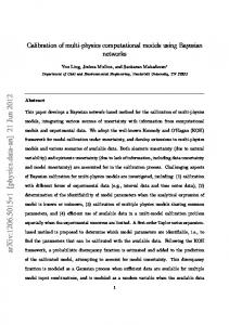
Fig. 1. Phase shift δ and its derivative dδ/dq as functions of squared momentum: (a) for the potential with two bound states; (b) for the potential with one bound and one semibound state.

(2)

= lim [ b 11 ∂ψ/∂r + b 12 ψ ] = 0, r→0

(3)

= lim [ b 21 ∂ψ/∂r + b 22 ψ ] = 0,

(44)

r→∞

where the functions bij , i, j = 1, 2, are defined by asymptotic conditions (42) or (43). For the Morse potential (n = 1) with two bound states (v = δ(0)/π = 2), phase shift δ and its derivative ∂δ/∂q as functions of squared momentum are shown in Fig. 1a. The accuracy of calculations and the quality of the functions ψ can be checked with the help of the derivative ∂δ/∂q, using the virial theorem [16] 2 2

crete analogue of the evolution method with respect to the coupling constant [14] or the Davidenko method [6]. For continuum problem (25), (26), (28), we can choose, for example, the parameter q, which is the value of momentum in the channel at some value of the spectral parameter λ (or energy 2E = q2), as a. Then condition (37) takes the form F ( q*, ψ ) = ( ψ, ( H – q* )ψ ) = 0, 2

(40)

similar to (28). In this case, iterations with respect to the parameter q in the vicinity of q = q* serve for determination of derivatives with respect to this parameter of interest. For illustration, we restrict ourselves to consideration of the problem of elastic scattering for models of quantum mechanical systems described by the radial Schrödinger equation on the half-axis ρ ∈ (0, ∞) with the short-range spherically symmetric potential V(ρ) ≡ V(ρ, g) (V(ρ) ≡ V(ρ, g = 0) ≡ 0) in the n-dimensional space for the given coupling constant g ≥ 0, momentum q ≥ 0, and angular momentum l (see [15]), 1 d n – 1 d l(l + n – 2) 2 ⎛ ---------- ------ρ ------ – ------------------------- + q ⎞ Ψl ( ρ ) 2 ⎝ ρ n – 1 dρ ⎠ dρ ρ

(41)

= V ( ρ )Ψ l ( ρ ). The corresponding boundary conditions for Eq. (41) are obtained by the transfer of asymptotic conditions for wave functions from the singular domain [0, ∞) l

Ψl ( ρ ) ρ → 0 ρ , –ν

Ψ l ( ρ ) ρ → ∞ Cρ sin ( qρ – π ( l + ν – 1 )/2 + δ l )

(42)

to the finite region of integration ρ ∈ [ρmin, ρmax], where ν = (n – 1)/2, δl is the sought phase shift, and C is the normalization coefficient. Problem (41) is considered on the whole axis (–∞, ∞) in the one-dimensional space (n = 1). Then, for the potentials with the asymptotic V(ρ) ρ → ±∞ exp(±ρ), it is convenient to use the following conditions instead of (42): Ψ ( ρ ) ρ → –∞ 0,

Ψ ( ρ ) ρ → ∞ C sin ( qρ + δ ).

(43)

Problem (41)–(43) is reduced to the finite interval [0, ρm] using the homogeneous boundary conditions

C q ∂δ/∂q = ( ψ, ( 2V + r∂V /∂r ) ). Another possibility studied in detail in [13] is the choice of the coupling constant g in (26) as a in (37). Then, condition (37) has the form 2

F ( g*, ψ ) = ( ψ, ( H ( g* ) – q )ψ ) = 0,

(45)

and, according to the Hellmann–Feynman theorem, it allows one to control the quantity ∂K/∂g = – ( ψ, ( ∂V ( g )/∂g )ψ )

(46)

and, under certain constraints on the potential V, to obtain one-sided estimates of elements of the K matrix [17]. Iterative schemes (37)–(39) can be applied for more precise determination of different variational calculations in the scattering problem. Indeed, the scattering problem for the Schrödinger equation with the above additional conditions can be reduced to calculation of the functional in the framework of different Hulthen, Kohn, or Schwinger variational principles. Thus, for example, for solution of the quantum problem of a few particles with short-range pair potentials, the Schwinger variational functional is used [18], and different iterative schemes have been developed on its basis. At first sight, the integral formulation of the problem is much simpler than the differential formulation, since it does not require detailed analysis of asymptotic behavior of the sought solution at g ≠ 0 for calculation of the functions bij , i, j = 1, 2 in (44), but uses only known regular and irregular solutions for g = 0. However, such schemes for the multichannel scattering problem do not provide stable calculation of the necessary physical parameters in a number of cases. Therefore, the development of stable variational–iterative schemes on the basis of the combination of projection methods, variational principles, and Newton iterative schemes is a topical problem of numerical modeling of quantum mechanical systems. 2.3.2. Multiparameter Newton iterative scheme with Schwinger functional. Boundary value problems (41), (42) are reduced to the spectral problem for the Fredholm equation [19]: A l ( ρ, ρ' )Ψ l ( ρ' ) = λ l B l ( ρ, ρ' )Ψ l ( ρ' ),


Vol. 38

No. 1

(47) 2007


A l ( ρ, ρ' )Ψ l ( ρ' ) ∞

∫

= Ψ l ( ρ ) – G l ( ρ, ρ' )V ( ρ' )Ψ l ( ρ' )ρ'

n–1

dρ', (48)

0 ∞

∫

B l ( ρ, ρ' )Ψ l ( ρ' ) = y l ( ρ ) y l ( ρ' )V ( ρ' )Ψ l ( ρ' )ρ'

n–1

dρ',

0

where λl = – π cot δ l /2 is the sought spectral parameter, and the dependence on the normalization coefficient C in the asymptotic of the unknown wave function Ψl (ρ) is eliminated. The function yl (ρ) and the free Green’s function Gl (ρ, ρ') are determined in terms of regular and irregular at the point ρ = 0 solutions to Eq. (41) for V(ρ) ≡ 0. The function yl (ρ) has the form –µ

y l ( ρ ) ≡ ρ J l + µ ( qρ ),

µ = n/2 – 1,

n > 1,

(49)

where Ji is the Bessel function of the first kind. The additional condition of the type (37) is used for solution of the problem (47), (48): ( V (ρ)Ψ l(ρ), ( A l ( ρ, ρ' ) – λ l B l ( ρ, ρ' ) )Ψ l ( ρ' ) ) = 0, (50) which implies the Schwinger variational functional ( V ( ρ )Ψ l ( ρ ), A l ( ρ, ρ' )Ψ l ( ρ' ) ) -, λ l = ----------------------------------------------------------------------( V ( ρ )Ψ l ( ρ ), B l ( ρ, ρ' )Ψ l ( ρ' ) )

(51)

where the brackets (·, ·) denote a scalar product, i.e., ∞ n–1 ( f, g) = 0 f *gρ dρ . As a result, integral equation (47) corresponds to the functional stable with respect to first order variations in Ψl , and scattering problem (41), (42) is formulated as the eigenvalue problem with respect to the pair of unknown functions z = (λl , Ψl ), the function of the phase shift λl and the wave function Ψl . Discretization of problem (47), (50) on a grid of nodes Ωh ∈ [ρmin, ρmax] (using known Bode’s quadrature formulas) results in the algebraic generalized eigenvalue problem

∫

( A – λB )Ψ ⎞ ϕ(z) = ⎛ = 0. ⎝ ( VΨ, ( A – λB )Ψ )⎠

(52)

Then, the iterative scheme for finding the approximations λk + 1, Ψk + 1, using the corrections vk, uk, and µk, is constructed: ⎧ v k = –Ψk ⎪ ⎪ ( A – λ k B )u k = BΨ k ⎪ ( Ψ k V , AΨ k ) ⎪ – λk ⎨ µ k = ----------------------------( Ψ k V , BΨ k ) ⎪ ⎪Ψ ⎪ k + 1 = Ψk + τk ( v k + uk µk ) ⎪ λk + 1 = λk + τk µk , ⎩ PHYSICS OF PARTICLES AND NUCLEI

(53)

where {λ0, Ψ0} is the initial approximation in the vicinity of the sought solution, and the condition of minimization of residual [12] is used for the choice of the iteration step τk, k = 0, 1, 2, …. The expression for µk coincides with Schwinger variational functional (51). The generalization of iterative scheme (53) for the multichannel scattering problem is given in [20]. In [21], the convergence of the proposed iterative scheme was demonstrated for elastic scattering problem (41)–(43) with the Morse potential (n = 1), Woods– Saxon potential, and the potential of the spherically symmetric rectangular well (n = 3). However, the scheme has the second order of accuracy with respect to the step h of the uniform grid Ωh, since the first derivative with respect to the argument ρ of the Green’s function Gl (ρ, ρ') has a singularity at ρ = ρ'. For the potentials considered, the phase shift δ was calculated to an accuracy within six decimal places. It was also shown in [21] that the application of the asymptotic Ψ(ρ) in the vicinity of the point ρmin for approximation of solutions allows the construction of schemes of a higher order of accuracy for calculation of the phase shift δ. The efficiency of the implementation of such sixth-order accuracy with respect to the step h scheme on the uniform grid Ωh was demonstrated by calculation of the phase shift δ to an accuracy of twelve decimal places for the one-dimensional scattering problem with the Morse potential. Corresponding algorithms are implemented in the form of program packages in Fortran with double-accuracy real numbers.1 2.4. Methods of Investigation of Localized Structures and Critical Modes in Nonlinear Problems Modern models of theoretical physics are described by complex systems of nonlinear partial differential equations allowing in some cases soliton or soliton-like solutions (localized in space particle-like states with a finite energy). Modeling of phenomena related to the formation, propagation, and stability of solitons represents a fast-developing interdisciplinary field of modern computational physics. The reason for the interest in this field is obvious—solitons and soliton-like formations are important examples of stable states in a very wide class of nonlinear unbounded and homogeneous models of physical systems (see, e.g., [22–25]). However, real physical systems are bounded in space and can have internal structural inhomogeneities contributing to the generation of new physical effects. The explanation of these effects is related, as a rule, to the possible localization of solitons on inhomogeneities and to their interaction with boundaries. If there is no external energy source in the system, and there exists damping related to energy dissipation, then an arbitrary 1 http://www.jinr.ru/programs/jinrlib/dll2;

jinrlib/scatterh6. Vol. 38

No. 1

77

2007

http:www.jinr.ru/programs/

78

PUZYNIN et al.

initial soliton state transforms into some equilibrium (static) solution, which is sometimes called [25] the static attractor. Self-similar solutions to nonlinear equations, for example, solutions of the type of traveling waves in a moving coordinate system related to the wave, can also be formally considered as “static” solutions. In the general case, homogeneous solutions mean static or time-periodic and quasiperiodic solutions. The considerable difficulties in the investigation of the stability of equilibrium solutions with respect to small space-time perturbations are determined by the presence in the models of given or unknown geometric and physical parameters—system dimensions and inhomogeneities, the structure of inhomogeneities, parameters defining the behavior of fields at the boundaries, the form and value of nonlinear interaction of elements of the system, and so on. In many classical models of physical systems, gradual change of a particular parameter corresponds to a unique continuous solution, and the linear stability theory describes the system states sufficiently well. However, there exist a large number of problems in which the number and stability of solutions change sharply upon the transition of a parameter through some critical values. Such phenomena, usually called branchings or bifurcations [26–28], can describe qualitative changes in a physical system. The values of the parameters for which bifurcation of solutions takes place are called bifurcation or critical values, and the process of transition through critical values of the parameters is called the critical, or bifurcation, mode. The geometric position of the points in the parameter space that correspond to the bifurcation of solutions defines in the general case some hyperplane called the bifurcation surface or the catastrophe surface [28]. In the theoretical aspect, the knowledge of bifurcation dependences allows the determination of the number of equilibrium solutions and the understanding of their structure, the estimation of the parameter ranges in which stability or instability of the system can be expected, and, possibly, the description of the physical phenomena occurring in this case [25]. The possibility of experimental verification of bifurcation dependences, which is an essential source of information for improvement of a model, is of special importance for practical purposes. Methods of investigation of vortex soliton-like structures of magnetic flux in long Josephson junctions (LJJ) based on measurement of (bifurcation) critical current as a function of magnetic field [29, 30] is a particular example. Unfortunately, analytical expressions for bifurcation surfaces can be obtained only in quite simple models. For the most interesting problems of modern theoretical physics, only numerical investigation of bifurcation dependences of parameters is possible. The traditional instrument for investigating the dependence of structural solutions on a parameter is continuation methods that are based on numerical

methods of solution of the Cauchy problem. However, in the vicinity of bifurcation surfaces, such methods are hardly applicable, since on these surfaces the uniqueness of solutions is violated. Therefore, the creation of numerical methods allowing one to find and study the behavior of solutions in the vicinity of bifurcations, and the construction of corresponding program packages implementing these methods is a very topical problem of mathematical modeling. 2.4.1. Continuation schemes with respect to parameters through a turning point. In this section, we present the general concept of numerical continuation with respect to a parameter and two continuation schemes, opening additional possibilities of numerical investigation. Originally, continuation methods were developed as a way of obtaining initial approximations in order to extend the region of convergence of iterative methods used for the solution of nonlinear problem (2) for a fixed set of parameters (see [31] and references therein). Modern developments in this field are aimed, to a large degree, at the solution of problems related to the analysis of bifurcations and critical modes in nonlinear problems (see, e.g., [32–34]). Any numerical continuation scheme contains, in some form, three obligatory components: (1) choice of initial approximation; (2) a method of solution of the problem for the given value of the parameter (the most widespread methods are Newton iterative schemes); (3) an algorithm of continuation with respect to the parameter. Note here that there exist algorithms uniting some of the above components in one iterative scheme. Such schemes include, for example, the method of parameter evolution (see [35] and references therein). The initial approximation is usually constructed using numerical results obtained at previous steps. The simplest and most widespread, and in many cases quite efficient, version of the continuation scheme is an organization of calculations for which the solution from the previous step is used as the initial approximation for the next value of the parameter. In order to provide higher stability and faster convergence of Newton iterations, the initial approximation is constructed on the basis of results calculated for 2–3 previous values of the parameter. Thus, the following Euler scheme is often used for the initial approximation: ϕ ( αi ) – ϕ ( αi – 1 ) (0) - . (54) ϕ (α i + 1) = ϕ(α i) + ( α i + 1 – α i ) -------------------------------------αi – αi – 1 Here, αi is the element of the parameter vector a at the ith continuation step. If the initial approximation is constructed at the starting point of the numerical continuation (i = 0), either an analytical form of solution known for some limiting values of parameters or qualitative information on its shape available for a majority of physical problems are used. In the framework of generalization of CANM, in some cases this problem is


Vol. 38

No. 1

2007


79

β

S(α)

(b)

(a)

α

α

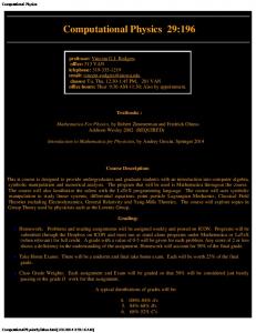
Fig. 2. (a) Continuation through the turning point with respect to parameter; (b) numerical continuation on the plane of parameters (α, β).

solved on the basis of representation of the function ϕ(t, z(t)) in evolution problem (6) in the form of sum (11) ϕ ( t, z ( t ) ) = ϕ 0 ( z ( t ) ) + g ( t ) [ ϕ ( z ( t ) ) – ϕ 0 ( z ( t ) ) ], where the operator ϕ 0' (z) is easily invertible, the solution to the equation ϕ0(z) = 0 is easily found, and the inclusion function g(t) is such that g(0) = 0, g(∞) = 1. Methods of choice of the step of continuation with respect to a parameter are determined by the specific features of particular problems and goals of investigation. One of the criteria of this choice is stable convergence of Newton iterations. If the step with respect to the parameter is sufficiently small, it is shown by corresponding theoretical estimates that the initial approximation lies in the region of convergence of Newton iterations. The step can be somewhat increased, and the continuation procedure can thus be accelerated by the choice of the iteration parameter τk in the Newton iterative scheme. The possible nonunique character of solutions and the presence of bifurcations require the development of special methods of numerical investigation. Thus, one of the problems of numerical continuation with respect to a parameter of solutions to nonlinear problems related to the nonunique character of the solution is the organization of continuation with respect to a parameter at the turning points where it is necessary to change the direction of continuation with respect to the parameter and pass over to a new unknown branch of solutions (Fig. 2a). The continuation algorithm presented in this section provides the solution to this problem. The idea of the proposed approach is as follows. If the solution z to the stationary boundary value problem ϕ ( z, α ) = 0

(55)

(where ϕ is the nonlinear operator, a is the element of the parameter vector a with respect to which the solution is continued, and the other elements of the vector a are fixed) is continued with respect to the parameter α, PHYSICS OF PARTICLES AND NUCLEI

Vol. 38

No. 1

one usually calculates the norm or another scalar characteristic of the solution S(z) (the so-called “measure of bifurcation”), and constructs its dependence on the parameter S(α). As a rule, quantities that have a physical meaning in the models considered are used as this scalar characteristic. In the continuation scheme proposed in [36], the fact that the derivative dα/dS(z) vanishes at the turning point is used. The position of the turning point at which the motion along the bifurcation curve should change direction can be found with the required accuracy by numerical approximation of this derivative and verification that the following relation is satisfied at each step with respect to the parameter: ∆α -----------i < , ∆S i

(56)

where > 0 is the predefined small number, ∆αi = αi – αi – 1 is the parameter step, and ∆Si = |S(z(αi )) – S(z(αi – 1))|. This means that if condition (56) is satisfied, the sign of the step of the continuation parameter should be changed to the opposite. In this case, the construction of the initial approximation by formula (54) using the results obtained for two previous values of the parameter excludes the return to the branch with the known solutions. The parameter step is calculated by the formula ∆S i – 1 ∆α i + 1 = ∆α i -------------, ∆S i

(57)

which provides its reduction in the vicinity of the turning point, where the solution changes quickly, and its increase on the “flat” interval of the bifurcation curve. In this case, the initial (i = 0) parameter step should be sufficiently small to provide stable and fast (in 3–5 iterations) convergence of the Newton iterative scheme. Note that on “flat” intervals of the bifurcation curve, “classical” Newton iterations are efficient, while at intervals near turning points it is necessary to pass over to iterations on the basis of CANM, which is provided by a corresponding choice of the iteration parameter τ. 2007

80

PUZYNIN et al.

Thus, the presented approach provides a possibility of passing over to new branches of solutions at turning points, preserves the structure of the matrix approximating the operator of the Frechet derivative and does not complicate, unlike other known recipes [32, 33], the Newton iterative scheme. On the other hand, the proposed algorithm of choice of the parameter step provides control of its value, and thus ensures fast convergence of Newton iterations and a high rate of continuation. In [37], another continuation scheme is presented. The modified continuation scheme with respect to the parameter with simultaneous calculation of another parameter is intended for realizing numerical continuation on the plane of two parameters, one of which is unknown (see Fig. 2b). The scheme combines the above continuation procedure with Newton iterations for the nonlinear functional equation ⎧ ϕ ( z , α, β ) ⎫ F ( z, α, β ) ≡ ⎨ ⎬ = 0, ⎩ Γ ( z, α, β ) ⎭

(58)

where β is the unknown element of the parameter vector a, and continuation is performed with respect to the parameter α, whereas other elements of the vector a are fixed. The additional condition Γ is formulated taking into account specific features of a particular problem, for example, on the basis of the variational approach [15], using the parametric dependence of solutions at the asymptotic [38], taking into account the translation invariance of solutions [37]. After the transition to the evolution equation and subsequent discretization with respect to the continuous parameter t, we obtain the iterative scheme of the following form at each step of numerical continuation with respect to the parameter α: zs + 1 = zs + τs φs ,

βs + 1 = βs + τs µs .

(59)

Here, s is the number of the Newton iteration, τs (0 < τs ≤ 1) is the iteration parameter of the Newton scheme, φs is defined as the linear combination φs =

(1) φs

+

(2) µs φs ,

where (1)

–1

φs

= – [ ∂ϕ/∂z ] s ϕ ( z s, α i, β s ), (2)

φs

(60)

–1

= – [ ∂ϕ/∂z ] s ∂ϕ/∂β,

and the iterative correction µs is calculated by the formula (1)

– Γ ( z s, α i, β s ) – [ ∂Γ/∂z ] s φ s -. µ s = -------------------------------------------------------------------(2) [ ∂Γ/∂z ] s φ s + [ ∂Γ/∂β ] s

algorithm described above. The initial approximation and the parameter step are calculated by formulas (54) and (57), respectively. 2.4.2. Linearization method in investigation of critical modes of nonlinear systems. In [39], the problem of calculation of bifurcation curves for equilibrium solutions of a wide class of nonlinear equations with the operator depending on some set of parameters is formulated. Let T be the interval on the real half-axis [0, ∞). We consider the particular form of Eq. (1), u˙ + G ( u, p ) = 0.

(61)

The real or complex-valued vector function u(t) (of dimension M ≥ 1) is defined on T and takes values in the Banach space with the norm ||·||. We denote by G the nonlinear operator defined on some set ⊂ and depending on the K-vector p ∈ ⊂ K of physical parameters of the model. Multiple examples of physical models whose equations are reduced to the form (61) can be found, for example, in [22–25, 27]. Equations of physical models considered in this work can also be written in the form (61). We assume that in some parameter range ∈ K, Eq. (61) has the equilibrium solution us(p) with a smooth dependence on the parameters, such that G ( u s, p ) = 0.

(62)

Equilibrium solutions include static solutions resulting from, for example, dissipation in the model [25], solutions of a wide class of problems in self-similar variables [40, 41], solutions of field theory problems with a time-oscillating phase and a static amplitude [24], and some others. Investigation of the local stability of equilibrium solutions with respect to small perturbations in the linear approximation results in the eigenvalue problem A ( p )ψ = κψ,

(63)

and the appropriate normalization condition is N [ ψ ] = 0.

(64)

Here, the linear operator A ≡ G u' is the Frechet derivative of the nonlinear operator G(u) at the point us ∈ , and N[ψ] is the given Frechet-differentiable functional. It will be assumed that in some region of the parameter space the spectrum of the operator A(p) is discrete. Let λ(p) = minReκi (p). Then, the stability condition of the equilibrium solution us(p) has the form λ(p) > 0. For λ(p) < 0, the equilibrium solution is unstable. The equation λ( p) = 0

The value of the parameter β serves as the measure of bifurcation upon numerical continuation. The motion through the turning point is simulated by the

(65)

defines the bifurcation surface of the solution us in the parameter space. For calculation of the bifurcation points, the system consisting of equation for equilibrium states (62), equa-


Vol. 38

No. 1

2007


tion of the linear eigenvalue problem (63), and normalization condition (64), is considered as the unified nonlinear functional equation for the functions u(p), ψ(p), and one of the K parameters p which will be denoted by ξ (without losing generality, we choose ξ ≡ p1). The other K – 1 parameters are assumed to be known. The eigenvalue of linear problem (63) is also assumed to be fixed (for example, equal to zero). Thus, this system transforms into the inverse eigenvalue problem for the parameter ξ. The continuous analogue of Newton’s method is used for solution of the nonlinear eigenvalue problem. At each step of the iterative process, two pairs of linear equations for the increments (U1, U2) and (Ψ1, Ψ2) of eigenfunctions are solved, A ( ξ )U 1 = – G ( u, ξ ),

(66)

A ( ξ )U 2 = – G ξ' ( u, ξ ), [ A ( ξ ) – λI ]Ψ 1 = – A u' ( ξ )ψU 1 – [ A ( ξ ) – λI ]ψ, [ A ( ξ ) – λI ]Ψ 2 = – A u' ( ξ )ψU 2 – A ξ' ( ξ ).

(67)

The correction P for the eigenvalue is found from the equation –1

P = – ( N' [ ψ ]Ψ 2 ) ( N [ ψ ] + N' [ ψ ]Ψ 1 ),

(68)

implied by normalization condition (64). If (uk, ψk, ξk) is the approximate solution to the problem at the kth iteration (k = 0, 1, 2, …), the next approximation (uk + 1, ψk + 1, ξk + 1) to the exact solution is calculated by the formulas

ψ

k

k

k

k

k

k

k

k+1

= u + τ k ( U 1 + P U 2 ),

k+1

= ψ + τ k ( Ψ 1 + P Ψ 2 ),

u

ξ

k+1

k

(69a)

k

(69b)

k

= ξ + τk P .

The set of algorithms for determination of the optimal step is presented in Section 2.2.4. In special cases, when the solution to problem (62) can be obtained analytically, calculation of the bifurcation points corresponding to this solution is reduced to the inverse eigenvalue problem, i.e., it is necessary to find the value of the parameter ξ for which the condition λ(ξ) = 0 is satisfied. Basic equations of the Newton iterative scheme for such problems have the form (67), (68), and (69b). In many models, Eqs. (66) and (67) represent boundary value problems for second order differential equations. A higher order spline collocation difference scheme was developed in [39] for the numerical solution of such problems. This scheme is simple in implementation on uniform and non-uniform grids, and allows a simple generalization to problems with discontinuous derivatives. An efficient method of solution of the occurring algebraic block diagonal system of equaPHYSICS OF PARTICLES AND NUCLEI

Vol. 38

No. 1

81

tions is given. The capabilities of the scheme are demonstrated on particular test examples. 2.5. Problem-Oriented Program Packages Table 1 shows program packages developed for numerical investigation of a number of problems. The software that turned out to be widely applicable is stored in the freeware electronic library JINRLIB (the corresponding products are written in bold letters). The majority of programs presented in Table 1 are constructed on the basis of different versions of the continuation method in combination with iterations by CANM and its generalization. 2.5.1. Program packages for solution of eigenvalue problems on the basis of CANM. (1) SLIP1 [42], for solution of the eigenvalue problem for a second order linear differential equation with boundary conditions nonlinearly dependent on the spectral parameter, with the finite-difference approximation O(h2).2 (2) SLIPH4 [43], a development of the SLIP1 package with a three-point approximation O(h4).3 Upon construction of the initial approximation of the solution, an algorithm on the basis of Newton’s method for finding roots of the polynomial with the exclusion of already found roots and the sweep method for higher stability of calculation of eigenfunctions was developed in [43]. (3) SLIPS2 [44], for solution of the eigenvalue problem for a system of two second order differential equations.4 (4) SNIDE [45], for solution of the eigenvalue problem for an integro-differential equation.5 (5) SYSINT (SYSINTM) [46], for solution of the eigenvalue problem for a system of integral equations.6 In the program, SYSINTM an iterative process is implemented in which the generalization of the operator of the derivative of a nonlinear function is replaced by two multiplications of linear operators at each iteration. The modified algorithm is more efficient for vector processors. For each package, a description of Newton iterative schemes and parameters of subroutines is given, specific features of program implementation are discussed, and examples of application of the package to the solution of physical problems are presented. (6) CANM [47], for solution of systems of nonlinear algebraic equations using CANM. 2.5.2. Program packages for investigation of nonlinear models of microprocesses. The program packages POLARON, DEUTERON, QUARKONIUM, 2 http://www.jinr.ru/programs/jinrlib/slip/#slip1. 3 http://www.jinr.ru/programs/jinrlib/slip/#sliph4. 4 http://www.jinr.ru/programs/jinrlib/slip/#slips2. 5 http://www.jinr.ru/programs/jinrlib/snide. 6 http://www.jinr.ru/programs/jinrlib/sysint.

2007

82

PUZYNIN et al.

Table 1. Program packages for numerical investigation of nonlinear models of microprocesses described by wave equations Package (program) TERM MATR TERM, MATR SLIP1, SLIPH4 SLIPS2, SYSTEM ITER, BAAP BSMADM SYSTEMQ SLIPH4

Problem (model)

Organization

Solution of the two-center problem in quantum mechanics; calculation of binding energy levels and wave functions of mesomolecules, mesomolecular complexes, quasistationary states, scattering on mesoatoms

Russian Research Centre Kurchatov Institute (Moscow), St. Petersburg State University (St. Petersburg), Institute of High Energy Physics (Protvino), Joint Institute for Nuclear Research (Dubna)

Calculation of energy levels of the

Joint Institute for Nuclear Research (Dubna)

+

antiproton pHe molecule CONTIN–NLIN CONTIN–NLIN–MOD PROGS2H4 GAO–EV CMATPROG OSCILLON PROGON4 POLARON SLIPS2 SNIDE, SLIPH4 DEUTERON MATPROG, SLIP1 QUARKONIUM SYSINT, SLIPS2 REL–SCHR SLIPH4, SYSINT HEA–CRS HEA–TOTAL DIRAC

Nonlinear Schrödinger equation

Joint Institute for Nuclear Research (Dubna), University of Cape Town (Republic of South Africa)

Stability of gap solitons

Joint Institute for Nuclear Research (Dubna), University of Cape Town (Republic of South Africa) Oscillons in the nonlinear Faraday res- Joint Institute for Nuclear Research (Dubna), University onance model of Cape Town (Republic of South Africa) Calculation of characteristics of opti- Joint Institute for Nuclear Research (Dubna), cal model of the polaron [4] Institute of Mathematical Problems of Biology, RAS (Pushchino) Quantum-field model of the binucleon Joint Institute for Nuclear Research (Dubna), Institute of Mathematical Problems of Biology, RAS (Pushchino) Quarkonium model on the basis of Joint Institute for Nuclear Research (Dubna) Schwinger–Dyson and Bethe–Salpeter equations [4] Relativistic model of quarkonium Joint Institute for Nuclear Research (Dubna) Calculation of characteristics of nuclear interactions in the framework of HEA Calculation of characteristics of elastic electron scattering

REL_SCHR for investigation of quantum field models include the already-mentioned programs SLIP1, SLIPH4, and SYSINT, in which CANM is implemented for the solution of various eigenvalue problems. In the CONTIN–NLIN7 and OSCILLON packages, the procedure of continuation with respect to a parameter through turning points is implemented. The package CONTIN-NLIN_MOD is composed using a modified continuation scheme on a plane of two parameters. The package GAP-EV is devoted to continuation with respect to a parameter of eigenvalues of a system of first order complex differential equations. The programs PROGS2H4,8 PROGON4,9 and MATPROG (CMATPROG)10 were developed for numerical solution of linear problems in calculation of 7 http://www.jinr.ru/programs/jinrlib/contin-nlin. 8 http://www.jinr.ru/programs/jinrlib/progs2h4. 9 http://www.jinr.ru/programs/jinrlib/progon4. 10http://www.jinr.ru/programs/jinrlib/matprog.

Joint Institute for Nuclear Research (Dubna), Institute of Atomic Energy (Poland), NCIAE (Egypt) Joint Institute for Nuclear Research (Dubna), INPAE (Bulgaria)

Newton iteration corrections. Such problems can serve as an object of investigation in various models. The necessity of their solution occurs, for example, in the framework of implicit schemes upon the solution of partial differential equations. The programs PROGON4 and PROGS2H4 [48] are devoted to the solution of, respectively, one and two ordinary differential equations with boundary conditions of the third kind. In both programs, the Numerov fourth order finite-difference approximation is used. The programs MATPROG and CMATPROG implement the matrix sweep method for real and complex variables, respectively. The program package HEA,11 including the programs HEA–CRS and HEA–TOTAL, is devoted to calculation of the characteristics of nucleus–nucleus interaction in the framework of the high-energy approximation. 11http://www.jinr.ru/programs/jinrlib/hea.


Vol. 38

No. 1

2007


The package DIRAC was developed for calculation of cross sections of elastic electron–nucleus scattering on the basis of the corresponding system of Dirac equations using the Message Passing Interface (MPI) technique for organization of parallel calculations.

Ψ ( r, R ) =

83

∑ Φ ( r; R )R J j

–1

J

χ j ( R)

j

+

∑ ∫ Φ ( r, R; k )R J s

–1

J

χ s ( R, k ) dk.

s

3. NUMERICAL INVESTIGATION OF MATHEMATICAL MODELS 3.1. Energy Levels of Mesomolecules in Adiabatic Representation of the Three Body Problem The problem of three quantum particles is a classical problem, and it is used as the model for description of physical processes in various fields: mesonic catalysis, antiproton capture in a mixture of helium atoms and hydrogen molecules, ionization of helium atoms by fast electrons and protons, nuclear fragmentation, and so on. Theoretical approaches to the investigation of these processes are closely related to computer modeling. Calculation with a required accuracy of energies and wave functions of helium and helium-like atoms, cross sections of the ionization reactions (e, 2e) and (e, 3e) of the helium atom by fast electrons, and investigation of reactions of simple proton capture p + He H + He+ and proton capture with ionization of the helium atom p + He H + He++ + e are topical problems for interpretation of new experiments in pulsed laser and electron spectroscopy in modern atomic physics. The development of stable and efficient methods of numerical analysis of the problem of three quantum particles is one of the fundamental problems of mathematical modeling of a wide class of physical processes. This section is devoted to the description of algorithms on the basis of the continuous analogue of Newton’s method and its generalization in the investigation of mesonic catalysis models, and main results obtained using these algorithms. The basic ideas of mesonic catalysis are presented in [49, 50]. The quantum mechanical three-body problem with Coulomb interaction is considered as the basic model. The parameters of such mesonic catalysis processes as charge transfer reactions with mesonic atoms, mesomolecule production rate, and attachment of mesons to helium are calculated by computation of characteristics of this system. It was noted that the model considered includes all basic quantum mechanical problems: the bound state problem, the scattering problem, and the inverse problem of reconstruction of nuclear interaction potentials from experimental data. The first approach in the investigation of these problems was the adiabatic representation [51] based on expansion of the wave function Ψ(r, R) of the original Schrödinger equation for the three-body system ( H – ε )Ψ ( r, R ) = 0 in the six-dimensional space (r, R) in a complete set of solutions to the two-center problem PHYSICS OF PARTICLES AND NUCLEI

Vol. 38

No. 1

Here, R is the vector between the nuclei of mesomolecules a and b (with the masses Ma and Mb, respectively, Ma ≥ Mb), r is the vector between the middle of the interval R and the µ meson (with the mass mµ). By applying the Kantorovich method to reduction of the partial differential equation, the following infinite system of ordinary integro-differential equations of the type (1) was obtained for Γ = 0: 2

J J d ⎛ -------- + 2Mε Jv – U ii ( R )⎞ χ i ( R ) ⎝ d R2 ⎠

=

∑ j≠i

J J U ij ( R )χ j ( R )

+

∑∫

J U is ( R,

J k )χ s ( R,

(70) k ) dk,

s

where M is the reduced mass of the system in mesoatomic units and –εJv is the binding energy of the vibrational state v of the system with the total angular momentum J. Thus, in this approach, it is necessary to implement a numerical scheme that would simultaneously provide an accuracy of calculation of the required characteristics depending on the number of terms of expansion, i.e., the number of equations of the system, and on the parameters of numerical approximation. It was shown in [52] that the Newton iterative scheme in combination with the continuation method with respect to particular parameters represents a promising and most optimal approach to the solution of this problem. The adiabatic representation includes expansion of the wave function Ψ in the set of wave functions of the two-center problem for the continuum and the discrete J spectra. This set and the effective potentials U ij (R) are found numerically. Control of the accuracy of calculations at each step is a complicated problem. For solution of this problem, numerical construction of the basis of the adiabatic representation of the threebody problem is considered. Statement of the two-center problem, algorithms of calculation of wave functions of the discrete spectrum and the continuum, and corresponding matrix elements are given in [53–56]. The concept of continuation with respect to parameters, in particular the coupling constant and the number of terms of expansion of the two-center wave functions in special bases, were implemented in numerical schemes. The asymptotic properties of wave functions and energies (terms) of the system at R 0 and R ∞ (R is a fixed distance between two centers) were used. 2007

84

PUZYNIN et al.

Taking into account asymptotic expressions for the sought wave functions of system (70), boundary conditions for nonlinearly energy-dependent wave functions of the discrete spectrum, the continuum, and the discrete-continuum (in the scattering problem with closed channels) spectra were formulated. Numerical approximation of the problem for system of radial equations (70) includes difference approximation of the differential operator in this equation and application of quadrature formulas of the same order of accuracy for the integral operator. In the 1970s, the first obtained results were those for the two-level approximation [54]. They were proved by the Vesman model of resonance formation of the ddµ mesomolecule [49, 50], and initiated investigations of the dtµ mesomolecule more promising for mesonic catalysis. Solution of large systems and extrapolation of the results with respect to the parameters of approximation was implemented using CANM and the continuation method. In the final adiabatic calculation [57] using 844 equations of system (70), the following nonrelativistic values of energy levels of weakly bound rotational–oscillatory states J = v = 1 of ddµ and dt µ mesomolecules were obtained: ε11(ddµ) = –1.956 eV, and ε11(dtµ) = –0.656 eV. 3.2. New Effective Potentials of Two-Level Approximation and Solution of Scattering Problem in a Three-Body System The adiabatic results stimulated direct variational calculations [58], since the development of computer power provided the possibility of carrying out complex calculations with completely filled matrices. Later, the more precise energy values –ε11(ddµ) = –1.97475 eV and –ε11(dtµ) = –0.6600 eV were obtained in variational calculations [59]. In these calculations, about 2660 variational functions of the discrete spectrum were used, and their form was chosen taking into account the specific features of the adiabatic expansion in the spheroidal coordinate system. Since the first results for the energy of weakly bound states of mesomolecules were obtained in the adiabatic representation, it was necessary to explain the above deviations. This is also useful for efficient application of adiabatic approximations in the muon three-body scattering problem, since other authors also solved it using an extended multichannel scheme [60] without taking into account the results obtained for bound states. The simple idea of constructing effective potentials of the two-channel approximation with a correct asymptotic reproducing energy levels of the discrete spectrum, which are at present accepted as the standard levels, yields an efficient scheme of calculation of the scattering problem and two-level wave functions of the discrete spectrum with the correct asymptotic behaviors [61].

The first adiabatic calculations were performed in the two-level approximation. In 1975, the quasistationary state of the dtµ molecule with the total angular momentum J = 1 and M = 10.894 was calculated (in these units, the reduced mass m* = 202.024me). For this mass, the energy –ε = E = 0.68 eV (E ≡ E˜ – E1(∞)) and the width Γ = 10.87 eV of this state were calculated. (1) The radial wave functions χ 1 (R) for the open channel (1)

and χ 2 (R) for the closed channel in the case of elastic scattering ( tµ ) 1s + d

( tµ ) 1s + d

(71)

are shown on the left-hand side of Fig. 3a. However, these results were not published in [62]. In [63], the transition of the quasistationary state of dtµ into the weakly bound state, where the mass M increases as a parameter, was reproduced. The right-hand side of Fig. 3b shows the energy E and width Γ as functions of this mass. For the mass M ~ 11.01, we have the state with zero energy and zero width, the so-called semi-bound state. The radial functions for this case are shown on the left-hand side of Fig. 4a. Function 1 of the open channel decreases slowly compared to function 2 of the closed channel. When the mass M increases, the system dtµ transfers into the bound state. For the mass M ~ 11.12, the “symmetric” energy value E = –0.68 eV was obtained. Therefore, it can be expected that the weakly bound state (J = 1, v = 1) exists, and the value of the binding energy is close to this value if we take into account all non-adiabatic corrections. Actually, our adiabatic multichannel and variational results are close to this value. If the function E is known, one can find for “exact” value E = –0.66 eV a corresponding effective mass value M ~ 11.11. Radial functions for this state are displayed in the right-hand side of Fig. 4b. These functions, unlike variational functions [64, 65], have a correct asymptotic behavior at R ∞. Thus, the variational energy level is reconstructed by the choice of the effective mass M = M(E) in the two-level approximation. The obtained results on modeling of the transition of the quasistationary state into the bound state resulted in the natural generalization of the effective mass M as the variable operator Θ (see (1), Γ = 0, Π = 0) in the new efficient two-level approximation [63]: 2

d d –1 ˜ ( R, M ) ) -----δMµ ( R ) ---------2 – δM ( 2Q dR dR J 2 ----- + V˜ ( R, M ) + p˜ χ˜ ( R, p˜ ) = 0.

Here, p˜ = 2M is the momentum matrix, δM = M/M is the correction matrix of the Jacoby M and adiabatic M ˜ (R, M) = Q(R) + (2M)–1∆Q(R), V˜ J (R, M) = masses, Q

V J(R) + (2M)–1∆V J(R) are the new effective potential


Vol. 38

No. 1

2007

METHODS OF COMPUTATIONAL PHYSICS χ 1.5

85

8 Γ

6

0.5 0 –0.5

20

40

60

2 –1.5

4

80 R

2 E

1

0

–2.5

11.15

10.95

M

–2 (1)

(1)

Fig. 3. (a) Radial wave functions (1) χ 1 (R) for the open, and (2) χ 2 (R) for the closed channels in the case of elastic scattering (tµ)1s + d with the angular momentum J = 1. (b) Energy E (eV) and width Γ (eV) as functions of effective mass M (tµ)1s + d for the dtµ mesomolecule.

χ 0.8

χ 0.8

0.6 1

0.4 0.2

0.4

2

0

20

40

60

–0.2

80 R

0

20

40

60

80 R

–0.4

–0.4 (1)

(1)

Fig. 4. (a) Radial wave functions (1) χ 1 (R) for the open channel, and (2) χ 2 (R) for J = 1 and zero binding energy ε = 0, (tµ)n = 1 + (1)

(1)

d (tµ)n = 1 + d. (b) Radial wave functions (1) χ 1 (R) and (2) χ 2 (R) of the ground state (J = 1, v = 1) of the dtµ mesomolecule.

matrices, and µ–1(R) = 1 + (2M)–1∆µ–1(R) is the inverse effective mass matrix µ(R) depending on the distance and satisfying the asymptotic conditions δMµ–1(R) 1 at R ∞. In this case, the corrections ∆Q(R), ∆V J(R), and ∆µ–1(R) are determined by the matrix elements J

Qij (R) and V ij (R) and the eigenvalues Ej (R) of the Coulomb two-center problem included in the definitions of the effective potentials of system (70). For example, the –1

diagonal corrections ∆µ ii (R) are determined in the form of the sum ∞

–1

– ∆µ ii ( R ) = 4

j≠i

∞

+

∑∫

s=0

Q ij ( R )Q ji ( R )

∑ -------------------------------------(E ( R) – E ( R)) i

j

(72)

Q is ( kR )Q si ( kR ) dk --------------------------------------. 2 ( E i ( R ) – k /2 )


Vol. 38

No. 1

If summation and integration in (72) is performed with respect to the complete set of states of the discrete spectrum and continuum of the Coulomb two-center problem, the asymptotic relation is satisfied due to the Thomas–Reiche–Kuhn sum rule. Since only a finite number of terms are taken into account upon summation, the asymptotic relation is not satisfied exactly. On the other hand, the following approximate relation is valid: µ–1(∞) = 1 – (2M)–1 × 0.5 ≈ 0.973, for (2M)–1 ≈ 0.05339 (exact value for ddµ). If only a finite number of states of the continuum are used in (72), we have the –1 following value: µ˜ (∞) ≈ 1 – (2M)–1 × 0.28 ≈ 0.985. This fact is explained by the specific features of the behavior of the matrix elements coupling the discrete spectrum and the continuum of the two-center problem [55]. Indeed, localization of matrix elements with increasing number l of the angular momentum of the muon shifts towards larger values of R [66]. Therefore, if we limit ourselves to a finite number of terms lmax upon summation with respect 2007

86

PUZYNIN et al. χ 1.5 1.0

1

2

2

1

0.5 0 –0.5 –1.0 –1.5 0

50

100

(1)

150

200 0 r

50

100

150

200 r

(1)

Fig. 5. (a) Radial wave functions (1) χ 1 (R) and (2) χ 2 (R) for J = 0 corresponding to (tµ) + d scattering with two open channels (2)

(2)

for the energy E = 0.3 eV; (b) Radial wave functions (1) χ 1 (R) and (2) χ 2 (R) for J = 1 corresponding to (dµ) + t scattering with two open channels for the energy E = 0.3 eV.

to l in (72), the contribution of the continuum ≈44% for ∞. As a result, we will l > lmax will be lost for R – 1 have |(µ–1(∞) – µ˜ (∞))/µ–1(∞)| ≈ 1%. In particular, the substitution of approximate values of effective masses for the fixed number of basis functions lmax at the point R0 < Rm (at the boundary of the region in which the effective potential acts) was necessarily used for calculations of the scattering problem with closed channels in [67]. It was shown in [63] that taking into account this circumstance upon formulation of the boundary value problem on the finite interval R ∈ [0, Rmax] for weakly bound states of ddµ and dt µ explains the relative difference, on the order of 1% between the variational and the adiabatic results. Thus, if an appropriate value of effective mass M = M(E) is chosen, we may limit ourselves to a finite number of terms upon summation in (72). Calculations of the cross section of reaction (71) using the corresponding values of M were performed [68] for verification of this approach. The radial wave (1) (1) (2) (2) functions χ 1 , χ 2 , and χ 1 , χ 2 , corresponding to (tµ)1s + d and (dµ)1s + t d + (tµ)1s the (tµ)1s + d reactions, are shown in Fig. 5. The results of the calcuJ lation of the partial ( σ 11 ) and total (σ11) cross sections of the elastic reaction of the tµ atom on the deuterium nucleus d (see Fig. 6) agree with other multichannel calculations [69] and reproduce the known shape of the resonance for J = 3 and E ~ 21 eV. 3.3. Structure of “Exotic” p He+ System In this section, the calculations of the structure of energy levels of the “exotic” p He+ system [70–73] are described. The energy level diagrams are shown in Fig. 7. Upon calculation of initial estimates of the energy of this structure in a wide range of quantum numbers, the

above idea of construction of new effective potentials of the two-level approximation reproducing the spectrometric experimental data [74] known with good accuracy due to the choice of fitting parameters [72] was used. This approximation allowed us not only to perform the required calculations efficiently, but also to obtain first estimates of fine and hyperfine structure and spin effects in the spectroscopy of the system [71, 73]. Experiments [74] using the effect of induced laser saturation showed that metastable states of the p He+ system have the quantum numbers nmax ~ 40, lmax ~ nmax – 1, corresponding to orbits close to circular ones, and the main initial population occurring at n ~ 38. However, an isolated system has a number of other populated metastable states in addition to these states. For explanation of the experiments, it was necessary, first of all, to calculate the initial populations and rotational–oscillatory states of the system. The characteristics of these states can be determined if the scheme of energy levels of the system is known. Here, we present the calculations of energy levels of the p He+ system using an effective adiabatic representation taking into account the nonadiabatic coupling [68, 70]. For investigation of the specific features of metastable states of p He+, different approximations were used for the formation of effective potentials in system (70). Here, we used standard definitions (see [75]), and the program [76] for calculation of the states of the discrete (D) spectrum and two types of approximations for determination of the states of the electron continuum spectrum (C) of the Coulomb two-center problem. The first approximation is the approximation of the united atom (UA) on the whole half-axis R, and the second approximation is the combination of the approximation of the united atom at small R and the approximation of the separated atom at large R. The second scheme with the separated atom (see [75]) was


Vol. 38

No. 1

2007

METHODS OF COMPUTATIONAL PHYSICS σ'11 , 10–20 cm2 80 60

87

σ11, 10–20 cm2 120 100

tµ + d – tµ + d

tµ + d – tµ + d

80

40

I=1

60

I=0

40

20

20 I=2

0 10–3 10–2 10–1 100 101 Energy, eV

0 10–3 10–2 10–1 100 101 Energy, eV J

Fig. 6. (a) Partial cross sections σ 11 (E), J = 0, 1, 2, 3, and (b) total cross section σ11(E) as functions of energy E for scattering of tµ atoms on the deuterium nucleus.

E –2.4

–2.8

p3He+

p4He+

–3.2

–3.6 30

40

35

45

50 30 J

35

3

J

40

45

50 J

4

Fig. 7. Energy levels E v (J = 30–50, v = 0–9) of (a) p He+ molecule, (b) p He+ molecule.

implemented. It will be shown below that application of these two approximations is sufficient for obtaining upper and lower estimates of the three-particle energy J

E v . The completeness of the chosen set of states corresponds to the contribution of the second order of the J

J

JBO

perturbation theory into ∆ E v = E v – E v , which was controlled by estimation of the corresponding Thomas– Reiche–Kuhn sum rule for effective potentials with the accuracy 10–5. In this case, 21 states of the discrete spectrum and 42 states of the continuum define the required effective potentials for system of radial equations (70). For the discrete spectrum, the corresponding basis elements {i = 1, …, 21} are correlated with the set of spherical quantum numbers (Nlm) of the united atom PHYSICS OF PARTICLES AND NUCLEI

Vol. 38

No. 1

{(m = 0, l = 0, N = 1), (m = 1, l = 1, N = 2), …, (m = 1, l = 1, N = 11), (m = 0, l = 0, N = 11). For the continuum, this sequence is complemented by the following subsequence: {i = 22, …, 63}: {(m = 1, l = 1, ε1), (m = 0, l = 0, ε1), …, (m = 1, l = 1, ε21), (m = 0, l = 0, ε21) with the same values of m, l, and electron energy εk = 0.5 tan x k , k = 1, …, 21, taken on the uniform grid ωh(x): (x1 = 10–8, xk + 1 = hk, k = 1, …, 20, h = 0.075, x21 = 1.5). Figure 8a J

shows the sequence of effective potentials U ii for J = 34. Note that the diagonal effective potentials with the numbers 22 and 23 corresponding to states with the zero energy (m = 1, l = 1, ε1) and (m = 0, l = 0, ε1) separate the continuum and the discrete electron spectrum of the two-center problem. 2007

88

PUZYNIN et al. Effective potentials UJii, a. u. –2.0

Emission rate Av'J'vJ, s –1 106

U40 40

–2.2

∆V = –1

J = 34 104

–1

U30 30

–2.4

U11

U22 22 U20 20 –3 U66

U44 U22

∆V = –2 V = 3...0

103 V=2

1

0

0.8

0.5

V=4 V=3

–2

–2.6 0.3

V = 3...0

105

U36 36

V = 0...4

1.0 R, a. u.

102

∆V = 1

32

34 36 38 Angular momentum J

J

Fig. 8. (a) Diagonal effective potentials U ii (R) for J = 34; (b) Rates Av 'J'vJ of some radiation transitions between states J'v ' Jv of p He+ ion (∆v = v ' – v, ∆J = J' – J).

The eigenvalue problem for the system of 63 coupled equations (21 states of the discrete spectrum and 42 states of the continuum) was solved using the Newton iterative scheme [58]. The sixth order finite-difference approximation of the boundary value problem with respect to the step h = hR of the uniform grid ωh(R) was used. This approximation was tested in [77] on an appropriate Coulomb two-particle (α particle and antiproton) problem for J ~ 30, i.e., for the antiproton helium atom in the final state after injection of the Auger electron which has the exact solution. Calculations were performed for 28 < J < 42 on the uniform grid ωh(R) = {R0 = 0.1; Ri = Ri – 1 + h, Rn = 1.5; i = 1, n} with the accuracy O(h6) for the step h = 0.00625. J

J

JBO

Figure 9 shows the differences ∆ E v = E v – E v J

comprised of the values E v of energies of the AD, DSA, SA, UA approximations (70) and the VK variational calculation [78] with respect to the BO approxiJBO mation E v (chosen here as the initial one) depending on the angular momentum J and the vibrational quantum number v = 0, 1, 2, 3. The DSA curves corresponding to calculations taking into account the discrete D electron spectrum only show that the asymptotic behavior of the contribution of the continuum C into the SA approximation is also correct and yields the upper estimate with respect to a more accurate curve VK representing the results of variational calculations [78]. It is seen that the BO approximation is satisfactory above JB = 37 and inadequate below this value. This is obvious, since for J < JB J

J

the diagonal effective potentials U 22, 22 and U 23, 23 separating the discrete and continuum electron spectra of the two-center problem are below the first SA threshold of the separated helium atom He+.

Another interesting point, JA = 32, corresponding to the lower metastable state, separates the region J < JA, where Auger processes prevail. It is seen that below this J point, the difference ∆ E v between the values of energy in the DSA and BO approximations is negative. This means that the BO approximation does not yield the lower estimate if the contribution of the continuum corresponding to Auger processes is not taken into account. This means that below JA the role of excitation processes also increases, i.e., JA is the lower boundary of the relatively long-lived metastable states. Thus, we determined the region of existence of metastable states JA < J < JB, inside which the BO approximation is not valid, and in order to obtain the adequate structure of levels and transitions between them, it is necessary to take into account nonadiabatic coupling. It can be concluded that taking into account nonadiabatic coupling in Eqs. (70) yields the upper and J lower boundaries of the shift ∆ E v with respect to the BO energy. This can be used for fitting experimental data for construction of an appropriate effective approximation of wave functions [79]. As an example, let us compare the theoretical values of the wavelengths corresponding to the UA approximation (without fitting) with experiment [74]: (3, 35) (3, 34): δE = 0.076288, λ = 597.255, (2, 35)

(2, 34):

δE = 0.086033, λ = 529.603, (2, 34)

exp. 597.259(2) nm, exp. 529.621(3) nm,

(2, 33):

δE = 0.096794, λ = 470.724,

exp. 470.724(2) nm.

Figure 8b shows the estimates Av 'J'vJ of the radiation transition rates similar to those obtained previously in


Vol. 38

No. 1

2007

METHODS OF COMPUTATIONAL PHYSICS 600 400

600

AD

0 –200

BO

0 –200

DSA

Energy difference ∆E [a. u.]

–600 SA VK

v=0 UA

–1200 600

0 –200

DSA

SA

–800

VK

–1000

UA

600

AD

∆E ×

AD

400

106

∆E × 106

200

BO

0 –200

DSA

–400

BO DSA

–400

SA

SA

–600

VK

–800

VK

–800

–1000

UA

–600

v=1

–1200

400 200

BO

–400

–600 –1000

∆E × 106

200

–400 –800

AD

400

∆E × 106

200

89

v=2

–1000

UA

v=3

–1200 –1200 30 31 32 33 34 35 36 37 38 30 31 32 33 34 35 36 37 38 Angular momentum J Angular momentum J J

J

JBO

Fig. 9. Energy differences ∆ E v = E v – E v calculated in the AD, DSA, SA, and UA approximations, and the variational VK calculation [78] with respect to the BO approximation as functions of angular momentum J and vibrational quantum number v = 0, 1, 2, 3.

BO approximation [80]. Estimates of energy levels and the transition dipole momentum calculated by the method presented here were used for construction of theoretical models of measurement and control of population dynamics of metastable states by laser pulses [81]. Note that this scheme of calculations taking into account nonadiabatic rotational–vibrational coupling of states with appropriate sets of electron quantum numbers (lm) also provides the required estimates of J

Wmin), Cv = 0.04 + 0.07v, v = 0, 1, …, 13, where Wmin = –0.0635974 and Wmax = –0.0629946 are the local minimum and local maximum of the potentials. The positions of the local minimum Rmin = 67.6 and local maximum Rmax = 47.6 are determined from the asymptotic expansion of the Rydberg term WNlm(R) in inverse powers of R. The radial wave functions in the external well corresponding to the minimum Ns = v + 1 = 1 and maximum Ns = 14 energy levels are shown in Fig. 10b.

the radiation transition rates Av 'J'vJ , energy levels E v , J

and widths Γ v for metastable states of the p He+ ion with the electron not only in the ground, but in the excited state as well [82, 83]. As an example, we mention Rydberg states of the antiproton helium atom in the so called Born–Oppenheimer approximation for the terms WNlm(R) corresponding to diagonal effective J

potentials U ii (R) for J = 0 without the diagonal nonadiabatic correction. For N = 6, l = 5, m = 0, this potential represented in Fig. 10a has 14 almost equidistant quasistationary states, whose energy levels are described by the approximate formula Eapprox = Wmin + Cv (Wmax – PHYSICS OF PARTICLES AND NUCLEI

Vol. 38

No. 1

3.4. Scattering Problem of Three Bosons on a Straight Line In nuclear physics, methods of bipolar and hyperspherical harmonics and single-parameter surface functions are widely used for correct solution of the problem of few particles with short-range pair interactions. In these approaches, the original problem is reduced by the Galerkin or Kantorovich method to spectral problems for systems of integro-differential or ordinary differential equations with the hyper-radius as an independent variable. Of special interest are problems with singular interactions, for example, centrifu2007

90

PUZYNIN et al. E –0.06275

0.5 Ns = 1

–0.06295

Wmax

0.3

Ns = 14

Ns = 14

–0.06315

0.1

–0.06335

–0.1

–0.06355

Wmin

–0.3

Ns = 1

W(R) × 5

W(R) = –2/R + E(R)

–0.5 –0.06375 20 40 50 60 70 80 90 100 R

40

60

80

100 R

Fig. 10. (a) Energy levels E in an external oscillatory well WNlm(R) for N = 6, l = 5, m = 0; (b) Wave functions for the lowest and highest energy levels.

gal interactions, interactions of zero radius in the form of δ functions, and problems with boundary conditions of the third kind. The issue is that the differential formulation of such problems causes difficulties. In order to avoid them, the problem is formulated as a system of integral equations, and in this formulation all difficulties are overcome by the choice of the appropriate parameter basis and approximation by the algebraic problem with completely filled matrices. Therefore, it is important to develop stable iterative schemes and algorithms of solution of spectral problems for systems of Fredholm integral equations. In [84], the developed algorithms are analyzed and tested on integrable models of three bosons on a straight line with zero radius pair interactions, since for these models the energy eigenvalues E of the bound and semi-bound states, and the S matrix of the processes of elastic scattering are known [86]. The phase shift and its derivative as functions of the squared momentum for the process of elastic scattering below the three-particle threshold E ≤ 0 is shown in Fig. 1b. For this model, the Schrödinger equation in polar coordinates ρ and θ for the partial wave function Ψi (ρ, θ) has the form [86] 1 ∂ ∂ --- ------ρ ------ – h ρ + 2E Ψ i ( ρ, θ ) = 0, ρ ∂ρ ∂ρ 1

ρ ∈ + ,

(73)

θ ∈ Ω.

Here, Ψi is the sought wave function, E is the energy in the center-of-mass system (in units = m = 1, where m is the boson mass), and hρ is the parametric Hamiltonian for each fixed value of ρ, 2

5

2g 1 ∂ h ρ = – -----2 --------2 + -----δ ( θ – θ n ), ρ ρ ∂θ n=0

∑

nπ π θ n = ------ + --- , (74) 3 6

where g = 2c κ is the coupling constant, κ = π/6, and c = –1 corresponds to the attraction of two particles and

ˆ is sought c = 1 to repulsion. The total wave function Ψ in the form of Kantorovich expansion in the orthogonal set of surface one-parameter functions Bj (ρ, θ) and as

∞, θ) with unknown coefficients

B j (θ) = Bj (ρ χji (ρ),

N–1

∑ |Ψ 〉 〈 B

ˆ = Ψ

i

as i |,

i=0 N–1

|Ψ i〉 =

(75)

N–1

∑ |B 〉 〈B |Ψ 〉 = ∑ B ( ρ, θ )χ j

j

i

j

j=0

ji ( ρ ).

j=0 1

The eigenfunctions Bj(ρ, θ) ∈ 2 (Ω) and the eigenvalues j (ρ) of Hamiltonian (74) are found for 1

each fixed value of ρ ∈ + from the boundary value problem 2

1 ∂ ⎧ – ---⎪ -2 --------2 B j ( ρ, θ ) = j ( ρ )B j ( ρ, θ ) ⎪ ρ ∂θ ⎪1 ∂ ± ⎨ --- ------ B j ( ρ, θ ) = − + cκB j ( ρ, θ n ), ± θ = θn ⎪ ρ ∂θ ⎪ πn ⎪θ ± = ±π --- + ------. ⎩ n 6 3

(76)

By averaging Eq. (73) with respect to the basis Bj(ρ, θ), we obtain the system of N ordinary differential equa1

tions on the half-axis ρ ∈ + of the type (41) for n = 2. The asymptotic boundary conditions with respect to the radial variable depend on the type of physical processes. For example, the asymptotic expression for the ∞ above the three-parradial functions χji (ρ) for ρ ticle threshold (E > 0) has the form


Vol. 38

No. 1

2007


Ψb 0.4 0.2

0

4

0 η

2

Ψhb 0.4 0.2 4 0 2 –0.2 –0.4 30

–2

0 ξ

–2

20

–4 –4

10

0 –10 ξ –20 –30

91

30 20 10 0 η –10 –20 –30

Fig. 11. Wave functions Ψb of the ground state and Ψhb of the semibound state for 2Eb ≈ 2Eexat = –π2/9 and 2Ehb, exact = –(π/6)2 (q = 0).

the solutions have a discontinuity. The elements of the K matrix below the three-particle threshold and in the region above the three-particle threshold were calculated to four and three decimal places, respectively, in the case N = 6. In [87], comparison with analytical results was made. Table 2 shows the comparison of the convergence rate of Kantorovich (75) and Galerkin

as

( – Y 1/2 ( qρ )δ 0i + J 1/2 ( qρ )W 0i ) ⎧ χ 0i ( ρ ) ⎪ as ⎨ χ ji ( ρ ) ( J 6 j – 3 ( kρ )δ ji + Y 6 j – 3 ( kρ )W ji ) ⎪ ⎩ for c = – 1, as

χ ji ( ρ )

(77)

( J 6 j + 3 ( kρ )δ ji + Y 6 j + 3 ( kρ )W ji ) for 2

c = 1, 2

Ψ i ( ρ, θ ) = ( 2π )

where q = π /36 + k , 2E = and Jj and Yi are the Bessel and Neumann functions of the first kind; Wji = k2,

– 1/2

χ0 ( ρ )

N–1

+ (π)

–1

K ji are the elements of the inverse matrix of the reaction. The corresponding two-dimensional scattering problem for Eq. (73) in the representation of oneparameter surface functions (75) is formulated as multichannel spectral problem (2) with respect to the pair of unknown variables z = (K, Ψ) for system of onedimensional integral equations (47) with matrix operators (48) and the additional Schwinger variational functional (50). The convergence of expansion (75) in the Kantorovich method and the efficiency of proposed iterative schemes (53) were demonstrated for the model considered below the three-particle threshold (E < 0) and in the region above the three-particle threshold (E > 0). It is seen from Figs. 11 and 12 that the wave functions have maximums for attraction (c = –1) and minimums for repulsion (c = 1) at the boundaries of six sections of the circle Ω, where the first and second derivatives of

– 1/2

∑

(78)

χ j ( ρ ) cos ( 6 jθ )

j=1

expansions, as exemplified by the calculation of the energy E(N) of the bound three-particle state for this model (c = –1). Slow convergence of ∆EG(N) with increasing number N of basis functions (78) is explained by the fact that the sufficient conditions of convergence of the classical Galerkin method cannot be weakened here. Moreover, thus reduced problem for any finite N has a false Coulomb spectrum with quantum defect and a qualitatively different threshold behavior of the phase shift [85] on the half-axis. This circumstance should be taken into account if the boundary value problem for the system of three particles with pair interactions allowing bound states is reduced by the Galerkin method.

Table 2. Comparison of convergence rates of Kantorovich (K) (75) and Galerkin (G) (78) expansions for calculation of energy E(N) of a bound three-particle state. The first row shows the number of equations N, the second and third rows show the difference ∆E(N) = E(N) – E exact of calculated E(N) and exact E exact values of energy N ∆EK ∆EG

1

2

3

4

5

6

1.801(–4) 9.662(–2)

2.762(–6) 4.116(–2)

2.697(–7) 2.573(–2)

5.413(–8) 1.866(–2)

1.594(–8) 1.462(–2)

5.949(–9) 1.201(–2)


Vol. 38

No. 1

2007

92

PUZYNIN et al. q = π/6 Ψ0s 0.2

Ψ0s 40 0 20 –0.2

0 –0.2 40

k = 0.6

0

20 ξ

0

–20 –20 –40 –40

η

40

40 20 0

20 ξ

0

–20 –20 –40 –40

η

s

Fig. 12. Scattering wave functions Ψ 0 for q = π/6 (for the three-particle threshold energy 2E = –k2 = 0) for attractive pair potentials (c = –1), and for k = 0.6 for repulsive pair potentials (c = 1).

3.5. Electron Correlation in Processes of Ionization of the Helium Atom Progress in the development of experimental methods of electron pulsed spectroscopy (EPS) (when at least two fast electrons measured in coincidence are produced in the reaction) achieved in recent years [88], in particular, the development of cold target recoil-ion momentum spectroscopy (COLTRIMS), allows precise kinematically complete investigations of complex atomic collisions [89]. Unique experiments on single and double ionization of atoms and molecules by fast electrons, performed by Japanese researchers in the EPS geometry, showed the necessity of both revision of the theory of the dynamical mechanisms of these processes, and the creation of a new family of variational wave functions as close as possible to the exact solution of the multiparticle Schrödinger equation for an atom or a molecule [90]. For this purpose, instead of the Lippmann–Schwinger equation with a noncompact singular kernel, resolventtype integral equations are formulated and investigated for the system of few particles with Coulomb interaction which have a connected kernel and in which all necessary singularities—two-particle (cluster) singularities and three-particle Coulomb singularities—are expressed explicitly. On the basis of such an approach, series of the perturbation theory are constructed in which higher Born terms describing interaction mechanisms are expressed by converging integrals and can be calculated numerically. A new method of construction of sample single-center wave functions of an atom with correlation functions explicitly depending on the distance between the electrons which reproduce the energy of the bound state with high accuracy and satisfy additional conditions of Kato type [91, 92] has been developed. This method is also applicable to molecules in the framework of the method of linear combination of atomic orbitals. The known two-center Coulomb wave functions [93] are used in calculations for the ion of the hydrogen molecule. The symmetry of

electron correlations of the molecular hydrogen ion and two atomic systems with two active electrons in ionization processes with excitation by fast electron impact was studied in the Born approximation using the quasiexact solutions in the basis of two-center Coulomb functions [94–96], which is necessary for adequate description of second order effects in experiment [89]. It is planned to test the above approaches and methods on the helium atom and hydrogen molecule and to use it further for the water and carbon oxide molecules that will be investigated by Japanese experimentalists. For the investigation of electron correlations, a new single-parameter basis of factorized correlated variational functions necessary for the calculation of energies and wave functions of bound states of helium-like atoms with a predetermined accuracy was constructed and examined in [97]. This problem, unlike the Coulomb two-body problem, does not have an exact analytical solution, but is the basic three-body system for precision calculations and experiments in atomic physics. For calculation of the energy of bound states, the variational Rayleigh–Ritz principle and an appropriate set of parametric trial functions in the coordinate representation are used. The upper estimate of the energy of helium atom in the ground state E = –2.903724377032 au in the nonrelativistic approximation for the infinite mass of the nucleus was obtained already in 1966 [98]. Recently, better estimates were obtained for the energy of this state, E = –2.903724377034119593 au [99] and E = –2.903724377034119597 au [100]. For explicit inclusion of the correlation of two atomic electrons at the distance r12 from each other, and at the distances r1 and r2 from the atomic nucleus, the perimetric coordinates r1, r2, r12 are used in variational calculations in [98]. In these coordinates, the radial part of the element of the integration volume is not reduced to a simple product of one-dimensional integrals; therefore, for transition to factorized correlated representation, it is necessary to use special projective coordinates.


Vol. 38

No. 1

2007


In [97], an alternative version of optimization of variational calculations was formulated, which provides a better stability and high accuracy of calculation of energy values. In projective coordinates, v = r 12 / ( r 1 + r 2 ),

s = r1 + r2 ,

(79)

w = ( r 1 – r 2 )/r 12

the three-dimensional integrals necessary for reduction of the variational problem to the algebraic problem are represented in the form of the product of one-dimensional integrals ∞

I =

1

∫ s ds ∫ v 5

0

0

1 2

∫

2

2

dv F ( s, v , w ) ( 1 – v w ) dw.

(80)

N

Ψ =

∑C ψ , n

n

(81)

n=0

ψ n ≡ ψ ij, 2k = U i ( s )V j ( v )W 2k ( w ), where W2k(w) are even functions of w on the interval [–1, 1] for the ground S state of helium-like atoms, in which all matrix elements of the Hamiltonian of the original problem with volume element (80) are calculated analytically. This problem, after variation of the Rayleigh–Ritz functional, is reduced to the generalized eigenvalue problem. For energy calculation, the Newton iterative scheme constructed on the basis of the variational Rayleigh– Ritz functional with the functions (81) in the form Ui(s) = Nie V j(v ) =

The corresponding program was written in Fortran, with double precision real numbers (in order to obtain up to thirteen decimal places accuracy in energy), and with four-fold precision (in order to obtain up to twenty two decimal places accuracy in energy). The results of numerical analysis of the convergence rate with respect to the number N in expansion (81) of the solution in the one-parameter basis of trial functions (82) were presented. Independent numerical calculation was performed, and comparison was made with the basis in projective coordinates not completely factorized [99] u = r> ,

( 0, 2 ) N j P j ( 2v

–αi s

– 1 ),

5

L i ( 2α i s ),

W 2k(w) =

(82) ( 1, 1 ) ˆ 2k P 2k N (w),

ˆ 2k are the normalization constants, where Ni , N j , and N ( q, t )

5

L i are the generalized Laguerre polynomials, P j are the Jacoby polynomials, and αi are the variational parameters, was used. The orthonormal basis Ui with the unique parameter α ≡ αi, whose value was determined from the condition ∂E(α)/∂α = 0, was used in calculations. In this approach, new upper estimates of the ground state of the helium atom were obtained to twenty two decimal places, E = –2.903724377034119598297 au, and new energy estimates for helium atom isotopes were obtained, E(He4) = –2.903304557733234397556 au, E(He3) = –2.903167210703584120495 au, and isoelectron states for Z = 3, …, 10. Note that calculations with multiparameter correlated exponential variational functions VK [101] for the ground state of the helium atom E = –2.903724377034119598311159 au confirmed our results. PHYSICS OF PARTICLES AND NUCLEI

Vol. 38

No. 1

v = r < /r > ,

r > = max ( r 1, r 2 ),

0

The main advantage of such a formulation of the problem is achieved by the choice of the correlated representation of the variational functions factorized with respect to all three arguments (79),

93

w = ( r 12 – r > )/r < , r < = min ( r 1, r 2 ),

(83)

for which Kato conditions in the form of boundary conditions at the point of pair electron collision are determined by the effective potential in the form of the δ function included explicitly in the definition of the Hamiltonian of the problem. In these coordinates, the radial basis function cannot be represented as the product of two radial hydrogen-like functions exp ( αs ) ≡ exp ( α ( r 1 + r 2 ) ) = exp ( α ( r > + r < ) ) = exp ( αu ( 1 + v ) ),

(84)

i.e., cannot be reduced to the exactly factorized form f( u )g( v ). In [102, 103, 90], models of processes of ionization of the S ground state of the helium atom by fast electrons and protons in the impulse approximation were investigated. Radial and angular electron correlations were studied, using known variational functions presented in [90]: the single-component Hylleraas function (Hy), the twelve-parameter Bonham and Kohl function (BK), Hylleraas–Eckart–Chandrasekhar (HEC), Hartree–Fock (HF), configuration interaction (CI), and the twelve-component (N = 12) single-parameter CVP function (81) constructed in [102]. The CVP function adequately takes into account electron correlation in the atom and agrees with the leading exponential term (84) in the asymptotic expansion of the formal solution of the “exact” wave function of the target [104] (see Fig. 13). Recently, the processes of double electron impact ionization of the helium atom, single ionization with simultaneous excitation, and double ionization were studied for a large value of the transferred momentum using the energy- and momentum-dispersion binary (e, 2e) spectrometer [90]. The experiment was performed for a collision energy of 2080 eV in the symmetric noncoplanar geometry. Thus, large momentum transfer, 9 au, i.e., a value that has never been achieved before in investigations of double ionization of the helium atom, was achieved. The measured cross sections of (e, 2e) and (e, 3 – 1e) for transitions to the excited (n = 2) He+ state and to doubly ionized He2+ state were normalized to the cross sections of transitions to the ground (n = 1) state of He+. The corresponding numerical results for 2007

94

PUZYNIN et al. Φ 1.0 0.6 0.2 0 0.5 1.0 1.5 r1 2.0 2.5

Φ

l=0

0

Φ

l=1

l=2 0.0015 0.0010 0.0005 0.002 0 0 0.2 0.2 0.4 0.4 0.6 0.6 0.8 0.8 r r 2.5 1.2 1 1 1.0 1.0 1.0 1.2 0.8 1.0 1.5 2.0 0.6 1.2 1.0 0.4 0.4 0.6 0.8 1.2 0 0.2 0.5 0.2 0 r 0.010 0.006

r2

r2

2

Fig. 13. Partial components Φl of the factorized twelve-component correlated variational function CPV (81) for electron angular momentum l = 0, 1, 2.

the normalized cross sections were obtained in the first order plane-wave impulse approximation (PWIA) and in the distorted-wave Born approximation (DWBA) using various wave functions of the ground state of the helium atom (with the purpose of investigation of models of the process dynamics and the structure of the quantum correlation of two-electron states). Figures 14a and 14b show the comparison of calculations of the (e, 2e) and (e, 3 – 1e) reaction cross sections with the variational functions Hy, HF, HEC, CPV, CI, BK; Fig. 14c shows the comparison with correlated exponential variational functions VK [101] taking into account Kato conditions both in the weak and strong sense [105], and experimental data. It is seen that the shape of the dependence of experimental cross sections of (e, 2e) and (e, 3 – 1e) on the transferred momentum is well-reproduced by PWIA calculations only when strongly correlated electron wave functions of the helium atom are used [90]. In [103], different models of the capture reaction were used, with ionization p + He H + He++ + e at very small hydrogen scattering angles θp = 0.1–0.5 mrad and the proton energy Ep = 0.15–0.14 MeV. It was proposed in [106] to use them in order to obtain new information on the structure of the wave function of the target in the impulse approximation. An assumption was made in [107] that upon construction of the theoretical model, the requirement of resonance capture can be omitted, and only the pole mechanism can be considered. However, in calculations with different variational functions and calculations with exact functions for the charge transfer reaction between the hydrogen atom and fast protons, second order effects should be taken into account for quantitative agreement with experimental data [108].

condensed states and nonlinear optics (see, e.g., [22] and references therein). In the framework of these models, an important problem is obtaining new information on the existence of stable particle-like states (solitons) in systems under study, on the conditions of occurrence of bifurcations and critical modes, and on the mechanisms of occurrence of instabilities. In nonlinear optics, for example, the occurrence of stable bound states of solitons is interpreted as the stable distortion of the signal, resulting in the loss of information in transmission lines and optical memory elements. The statement of the problem represents different versions of the complex-valued partial differential equation with a cubic nonlinearity and terms modeling dissipative energy losses and external energy pumping into the system. The following equations are considered. The nonlinear Schrödinger equation with the parametric pumping and dissipation 2

iΨ t + Ψ xx + 2 Ψ Ψ – Ψ = hΨ – iγΨ, Ψ ( x = ± ∞ ) = 0.

(85)

Hereinafter, Ψ is the amplitude of the quasi-harmonic stationary wave, h is the pumping amplitude, γ is the dissipation coefficient, and the bar above Ψ means complex conjugation. This equation is used in the description of magnets in a rotating magnetic field, in the theory of Josephson contacts, in hydrodynamics models, and in the analysis of microwave propagation in plasmas. In the case of direct (external) pumping, the Schrödinger equation has the form 2

iΨ t + Ψ xx + 2 Ψ Ψ – Ψ = – h – iγΨ, 3.6. Soliton Solutions to Nonlinear Schrödinger Equation with Dissipation and Pumping The nonlinear Schrödinger equation describes the amplitude of the quasi-monochromatic wave propagating in the nonlinear dispersion medium, and, as such, has many physical applications (in various mathematical formulations) in different models of the theory of

Ψ x ( x = ± ∞ ) = 0.

(86)

This equation describes the effect of phase amplification in optical fibers, convection in binary mixtures and liquid crystals, and magnetization waves in ferromagnetic materials under the action of a combination of a static and microwave fields, as well as having a number of other applications.


Vol. 38

No. 1

2007

METHODS OF COMPUTATIONAL PHYSICS He+(n = 2)

10–5

7 1

10–6

2 1 × 10–5 3 5 × 10–6

4–7 1

0

Four-fold differential cross section, a. u.

Triple differential cross section, a. u.

3 4–6

He2+(a) E3 = 10 eV

1 2

(e, 2e) n = 2

10–5

4 5 6

10–6

10–6

3 10–7 1 2

(e, 3–1e)

10–6

10–6

4 5 6 3

10–7

1 2 Momentum, a. u.

He2+(b) E3 = 20 eV

4DCS, a. u.

2

95

0

10–7 1 2 Momentum, a. u.

0

0.5 1.0 1.5 2.0 2.5 3.0 q, momentum, a. u.

Fig. 14. Comparison of experimental three- and four-fold differential cross sections of the processes (e, 2e) and (e, 3–1e) as functions of transferred momentum with theoretical calculations in PWIA and DWBA for different variational functions: (1) PWIA/Hy; (2) PWIA/HF; (3) PWIA/HEC; (4) PWIA/CPV; (5) PWIA/CI; (6) PWIA/BK; (7) DWBA/CI and PWIA/VK with Kato condition in the (1) strong and (2) weak form. See the text for detailed explanation.

Finally, for the case of nonlinearity of the defocusing type, the following equation is considered: 1 2 iΨ t + --- Ψ xx – Ψ Ψ + Ψ = hΨ – iγΨ, 2 Ψ x ( x = ± ∞ ) = 0,

(87)

which, in particular, models magnetization waves in easy-axis ferromagnetic materials with additional weak anisotropy. In gas dynamics, this equation is known as the equation of the amplitude of oscillations of the surface of a liquid in a vertically vibrating channel with large width and small depth. In nonlinear optics, Eq. (87) was obtained in the model of the optical parametric oscillator in a quadratic medium in the limit of large second harmonic offset. Numerical investigation of each of these three equations included: (1) continuation of stationary solutions with respect to a parameter; (2) numerical solution of the linearized eigenvalue problem for investigation of the stability properties of stationary solutions (for the above equations, this problem represents the system of two second order differential equations in complex variables); and finally, (3) numerical solution of the original partial differential problem for determination of the values of parameters. Numerical continuation of stationary solutions with respect to a parameter was performed using the proPHYSICS OF PARTICLES AND NUCLEI

Vol. 38

No. 1

gram CONTIN-NLIN. In most cases, numerical experiments were performed on the interval x = [–100, 100] with a step of the finite-difference approximation of 0.005. The linearized eigenvalue problem was solved using the standard program in the EISPACK library.12 Eigenvalues were refined by using the Newton iterations, if necessary. The original partial differential problem was solved numerically on the basis of the two-step conditionally stable algorithm with a Fourier approximation in the spatial variable [109, 110] known as the pseudo-spectral method. The goal of the investigation was the search for new classes of localized solutions in the form of multisoliton complexes and moving solitons, the study of the boundaries of the region of existence of localized states, the study of bifurcation points, and the numerical analysis of stability of soliton solutions. Two single-soliton solutions are known in the literature for each of Eqs. (85) and (86): for Eq. (85) they are known explicitly, and for Eq. (86) they are found numerically [111]. As regards multisoliton solutions to Eq. (85), although the bound states of solitons were observed in experiments on Faraday resonance on the surface of a liquid [112], theoretical analysis [113, 114] did not 12http://www.netlib.org/eispack.

2007

96

PUZYNIN et al. 1.0

γ = 0.565, h = 0.9

1.0 0.5

0.5

0

0

–0.5 –10

–5

0

5

–0.5 γ = 0.52, h = 0.35 –50 0

10 x

50 x

Fig. 15. Stable two-soliton complexes of (left) Eq. (85) and (right) Eq. (86). Solid lines correspond to the real part, and dashed lines to the imaginary part.

reveal the existence of bound states even in the case of strong overlapping of solitons. Multisoliton solutions of Eq. (85) were first found numerically and studied in [115]. In this work, an analytical approximation of two-soliton solutions was constructed on the basis of the variational approach. Two- and three-soliton complexes of Eq. (86) were first discovered in [116]. Unlike in Eq. (85), in (86) solitons can be coupled at different distances (“quantum orbits”), which is explained by their oscillating asymptotic behavior [117]. Numerical investigation of multisoliton complexes of Eq. (86) as functions of parameters was performed in [36]; in particular, stable two-soliton solutions were found for the first time. The region of existence of solitons of Eq. (86) was studied in [118].

0 y = ( λ + γ )J y, ⎛

0 = ⎜⎜ ⎝

2

Figure 15 shows stable two-soliton complexes first discovered for Eqs. (85) and (86). In [119], solitons of Eq. (85), where ψ(ξ) 0 at |ξ| ∞, moving with constant velocity, were investigated. Such solutions satisfy the ordinary differential equation 2

– iV ψ ξ + ψ ξξ + 2 ψ ψ – ψ = hψ – iγψ,

in which V plays the role of the additional parameter. The stability of moving solitons to small perturbations of the amplitude λt

δψ ( ξ, t ) = e [ δu ( ξ ) + iδv ( ξ ) ]

2

V ∂ ξ – 4uv

The stability criterion is the absence of eigenvalues λ with a positive real part. In the case of the zero dissipation, numerical investigation of moving solitons is performed by the same scheme which is used for immobile solitons, using the package CONTIN-NLIN. The case of nonzero velocity and nonzero dissipation is more complicated. For this case, necessary and sufficient conditions for bifurcation points, where branches of moving dissipative solitons originate, were formulated in [120]. These conditions were verified numerically. Soliton solutions were continued numerically from the found bifurcation points on the parameter plane (γ, V) and (h, V) using the package

(89)

is studied by numerical solution of the linearized eigenvalue problem, which in this case has the form

⎛ ⎞ J = ⎜ 0 –1 ⎟ , ⎝ 1 0 ⎠

–∂ ξ + 1 + h – 6u – 2v

(88)

2

T

y ( ξ ) = ( δu, δv ) ,

(90)

⎞ ⎟. 2 2 2 ⎟ –∂ ξ + 1 – h – 6v – 2u ⎠ –V ∂ ξ – 4uv

(91)

CONTIN-NLIN-MOD. It was shown that in the presence of parametric pumping, two or more dissipative solitons can form a complex moving with the zero momentum but nonzero velocity. Some results of numerical continuation are shown in Fig. 16. Localized states of Eq. (87) are called “dark solitons” in models of nonlinear optics and “domain walls” in models of the theory of ferromagnetism. As in the previous cases, localized solutions to this equation of a kink-like form—“Néel wall” and “Bloch wall”—are known explicitly in literature. One more known type of localized solutions to the equation with the defocusing nonlinearity is “bubbles.”


Vol. 38

No. 1

2007

METHODS OF COMPUTATIONAL PHYSICS γ 0.6

97

γ 0.7

0.4

h = 0.7

0.5 V = 0.651 γ = 0.346

V = –0.1898 γ = 0.3401

0.3

0

0.2

0

0.1

0

0.1

h = 0.8353 0.3

0.5

0.7

0

–0.8

–0.6

–0.4

–0.2

0

Fig. 16. Results of numerical continuation of dissipative moving solitons of Eq. (88) on the parameter plane (V, γ). Insets illustrate the solution at one of the internal points of the curve. Solid line corresponds to the real part, and dashed line to the imaginary part. The direction of numerical continuation is shown by arrows.

In [121], the inverse spectral problem generated by the family of analytic “bubble solitons” of the nonlinear Schrödinger equation is studied. A particular solution from this family is defined by two parameters A and V. The first parameter characterizes the medium in which the soliton moves, and the second parameter is the velocity of the soliton. The soliton is stable if its velocity is larger than some critical value depending on the parameters of the medium. The mathematical formulation of the problem is reduced to determination of the velocity of the soliton for which the eigenvalue of the corresponding linearized eigenvalue problem vanishes. The numerical investigation was performed on the basis of the two-dimensional approach described in Section 2.4.2. It was shown that the critical velocity of the soliton increases monotonically with increasing parameter of the medium. In [122, 123], new stable dissipative multisoliton complexes of Eq. (87) and, for the case of zero dissipation, branches of stable moving dark solitons were obtained. The effect of “multistability,” i.e., the coexistence of different types of stable states for the same sets of parameters was discovered. An example of the stable complex of two dark solitons is given in Fig. 17a. Figure 17b demonstrates the region of existence and stability of such solutions on the parameter plane (h, γ). In [124, 125], the lattice model of the nonlinear Faraday resonance is considered. The nonlinear equation with parametric pumping and dissipation for the amplitude of oscillating objects (oscillons) experimentally observed on the surface of a liquid and granulated materials was formulated in the framework of this model. The equation has the form 2

2

iψ t + ∇ ψ + 2 ψ ψ – ψ = hψ – iγψ.

(92)

Here, γ and h are the dissipation coefficient and the pumping amplitude, respectively (in the one-dimensional case we obtain (85)). Radially symmetric localPHYSICS OF PARTICLES AND NUCLEI

Vol. 38

No. 1

ized solutions to this equation in the two-dimensional and three-dimensional cases are considered. Two linearized eigenvalue problems were formulated for investigation of the stability of stationary oscillons to radial and azimuthal amplitude perturbations. Numerical investigation was performed using the package OSCILLON. As a result of numerical analysis, the parameter range in which two-dimensional oscillons are stable was found, and the corresponding diagram was constructed in [124]. The numerical results agree with theoretical investigations in the framework of the variational approach and with the results of direct computer modeling of the original partial differential equation (92) [125]. 3.7. Optical Fiber Model with Periodic Refractive Index The propagation of a traveling wave in optical fibers with periodic refractive index is described by the system of amplitude equations 2

2

2

2

i ( u t + u x ) + v + ( v + ρ u )u = 0, i ( v t + v x ) + u + ( u + ρ v )v = 0.

(93)

Here, x is the coordinate along the lattice, t is time, and ρ is the parameter taking values from zero to infinity in different models. (Note that system (93) has many other applications in different models of elementary particle physics and physics of condensed states.) Stationary soliton solutions to this systems (gap solitons) with the boundary conditions u(x = ±∞) = v(x = ±∞) = 0 have an explicit form and depend on the velocity V and angle θ (0 < θ < π) parameterizing the soliton frequency in the spectral range Ω = cosθ. The problem of stability of localized solutions to system (93) has been open for a long time, although many publications from the late 1970s, were devoted to it. Since the mid-1990s, interest in this problem has 2007

98

PUZYNIN et al. h 1.0

(a)

0.6

(b) 0.8

0.2

0.6

–0.2

E

–0.6

4

0.4

γ = 0.35

2

–1.0

0

0.2

–15

–10

–5

0

5

10

15

0.1

0.3

0.2

0.4

0.5

0.4

0.5

0.6

0.6 h

0.7 0.8

Fig. 17. (a) Example of a stable bound state of two dark solitons of Eq. (87) for γ = 0.35, h = 0.617. Solid line corresponds to the real part, dashed line to the imaginary part. (b) Region of existence of dissipative two-soliton solutions. Shaded area corresponds to stable solutions. The inset shows energy E as a function of h for the fixed value of γ. Solid and dashed lines show the stable and unstable branches, respectively.

increased due to the development of new technologies of information transfer and the investigation of corresponding nonlinear-optical models [126, 127]. An answer to this question was obtained in [128, 129]. In order to investigate the stability of slit solitons by linearization of the original system (93), the following eigenvalue problem for the system of four first-order differential equations in complex variables is formulated: ˆ z = λJz,

⎛ σ 0 ⎞ J = ⎜ 0 ⎟, ⎝ 0 –σ0 ⎠

(94)

T

z = ( z 1, z 2, z 3, z 4 ) , ⎛ σ3 0 ⎞ d ⎟ ------⎝ 0 – σ 3 ⎠ dX

ˆ = i⎜ ⎛ σ 0 +⎜ 0 ⎝ 0 σ0

⎞ ⎛ σ 0 ⎞ 2 ⎟ ( W + cos θ ) + ⎜ 1 ⎟ ⎠ ⎝ 0 σ1 ⎠

⎛ 2y 2 2 2y 2 2 –W ρe W –W ⎜ ρe W ⎜ –2 y 2 2 –2 y 2 2 2 –W ρe W* + α ⎜ – W* ρe W ⎜ 2y 2 2y 2 2 2 –W ρe W – W* ⎜ ρe W* ⎜ 2 –2 y 2 2 –2 y 2 ρe W –W ρe W ⎝ –W

⎞ ⎟ ⎟ ⎟. ⎟ ⎟ ⎟ ⎠

(95)

Here, σ0, σ1, and σ3 are the Pauli matrices. The indication of stability is the absence of eigenvalues with a positive imaginary part.

(1) Expansion of solutions in the Fourier basis and solution of the obtained eigenvalue problem using standard programs from the EISPACK library. (2) Refining and continuation with respect to a parameter of the eigenvalues most interesting from the point of view of stability. For this purpose, the program package GAP-EV was developed. In this package, the Newton iterative scheme using the finite-difference fourth-order Numerov approximation is implemented in the framework of continuation with respect to a parameter. (3) Numerical solution of the nonlinear algebraic system formulated in the framework of the perturbation theory for analysis of oscillatory instability in a particular parameter range, using Newton iterations. The results of numerical continuation of eigenvalues of problem (94) with respect to the parameter θ for fixed ρ and V are shown in Fig. 18. As a result of numerical investigation, the diagram of regions of instability in the whole parameter range was constructed (Fig. 19). The results obtained in [128, 129] agree with theoretical analysis and results of computer modeling for separate values of parameters in [130, 131]. Further, these results were corroborated in theoretical and numerical investigations of other authors (see, e.g., [132]). 3.8. Nuclear Interactions in High-Energy Approximation The motion of an incident nucleus with the kinetic energy E in the field of the complex nucleus–nucleus potential U is described by the Schrödinger wave equation 2

The following methods were used for numerical investigation:

-------∆Ψ + ( E – U )Ψ = 0. 2m


Vol. 38

(96) No. 1

2007

METHODS OF COMPUTATIONAL PHYSICS Reλ 2

lmλ 0.2

(a)

(b)

λ2(0)

λ1(0)

θosc θ2

ρ = 0.5, V = 0.9 θtr π

π/2

0

–0.2

θ2

θosc

0

1

99

θtr 3 2

1

π/2

0

π

− cosθ. A real eigenFig. 18. The numerically calculated eigenvalues. Dashed lines show boundaries of the continuum, λ1, 2(0) = 1 + value is detached from λ1 for θ = 0; another real eigenvalue is detached from λ2 for θ = θcr > π/2 (not seen in the figure). For θ = θosc two eigenvalues merge and form a complex conjugate pair, thus producing an oscillatory instability. Another complex pair is detached from λ1 for θ = θ2. Finally, one more eigenvalue is detached from λ2 and transfers to the imaginary axis for θtr.

V 1.0 1

2

Stable

2 0.5

0 –1.0

–0.5

1

3

0 Ω

–1.0

–0.5

Stable

3

0 Ω

Fig. 19. Stability diagram for (left) ρ = 1/2 and (right) ρ ∞ on the parameter plane (V, Ω = cosθ). Curves 1, 2, and 3 correspond to occurrence of “unstable” eigenvalues with positive imaginary part in the discrete spectrum. Dashed line shows asymptotic approximation of the original oscillatory instability.

Here, m is the reduced mass, Ψ(r) is the wave function of relative motion of the nuclei, and is the Planck constant. In the general case, the potential U depends on Ψ, and the problem is essentially nonlinear. One of the important problems in the investigation of Eq. (96) is the problem of construction of the potential U. Knowledge of the potential as the basic characteristic of nuclear interaction is necessary for the calculation of differential cross sections of elastic and inelastic scattering, and for the modeling of reactions of nucleon transfer. Of special importance is the method of construction of the imaginary part of the potential, since, to date, the basic theoretical works have been devoted to microscopic calculations of the real part of the functional, whereas its imaginary part is traditionally reconstructed by fitting free parameters. In order to provide the possibility of predictive calculations on the basis of numerical analysis of the available experimental data, generalized dependences of the parameters of the potentials on energy and the physical parameters defining the structure of colliding nuclei are PHYSICS OF PARTICLES AND NUCLEI

Vol. 38

No. 1

constructed. Such calculations were performed, for example, in [133]. Another known approach is based on construction of the dependence of nucleus–nucleus potential on the distribution function of the density of nuclear matter in nuclei. Information on this distribution function can be obtained from independent experiments. For construction of the real part of potentials, the double folding model (DF) is most widely used (see, [134] and references therein). In the framework of this approach, a nonlinear problem for an integral equation is formulated and solved by iterative methods for construction of the potential. As regards the construction of the imaginary part of the potential, one of the most efficient approaches is based on application of the high-energy approximation [135–137]. In the framework of the high-energy approach (HEA), when E |U| and the motion of the incident nucleus is close to free motion, the solution Ψ is approximated using functions of a special form called eikonal functions. This provides analytical expressions 2007

100

PUZYNIN et al.

for the differential cross section of elastic nucleus– nucleus scattering and for the total reaction cross section [138, 139], ∞ 2 dσ ------- = f ( q ) , dΩ

∫

σ r = 2π dbb [ 1 – e

– 2Im Φ ( b )

], (97)

0

where the elastic scattering amplitude f(q) and phase Φ(b) have the form ∞

∫

f ( q ) = ik dbbJ 0 ( qb ) [ 1 – e

iΦ ( b )

∫

Here, ρ˜ °i (q) (i = p, t) are the Fourier images of the point (98)

1 2 2 Φ ( b ) = – ------- dzU ( b + z ). v

∫

–∞

Here, q = 2ksin(θ/2) is the transferred momentum, θ is the scattering angle, k is the momentum, v is the velocity of the incident nucleus, J0 is the cylindrical Bessel function, and U(r) = Uc(r) + UN (r) is the potential including the Coulomb Uc(r) and the nuclear UN (r) = V(r) + iW(r) components. Thus, calculation of the basic physical characteristics is reduced either to numerical solution of Eq. (96), or to numerical or analytic integration of expressions (98), whose particular form depends on the way of construction of the potential U. The model on the basis of the high-energy approximation using approximate analytical expressions reducing the dimension of the original integrals and fundamentally simplifying the calculations, is implemented in the program package HEA-CRS and HEA-TOTAL. The numerical investigation proved the applicability of this approach to the modeling of nucleus–nucleus interactions at energies from 10 to 100 MeV per nucleon of the incident nucleus. At present, the program package is used for the processing of experiments performed at the Laboratory of Nuclear Reactions of the Joint Institute for Nuclear Research [140]. In [141], an approximate analytic method was proposed, and on the basis of this method an explicit expression for the phase Φ(b) was obtained for a phenomenological potential that is typical in nuclear physics; it is in the symmetrized Woods–Saxon form U N ( r ) = ( V 0 + iW 0 )u sf , sinh ( R/a ) u sf = --------------------------------------------------------, cosh ( R/a ) + cosh ( r/a )

∞

σ NN - dqqJ 0 ( qb )ρ˜ °p ( q )ρ˜ t° ( q ) f N ( q ). (100) Im Φ N ( b ) = -------2 0

],

0 ∞

of the original equation (96), and with experimental results in a wide range of atomic masses and energies. In [142, 143], methods of calculation of total cross sections of reactions were developed. In the framework of the microscopic approach, the imaginary part of the nuclear phase ΦN (b) in formula (97) is determined as follows:

(99)

with given parameters R and a. By replacement of typical integrals with specially fitted parametric expressions, explicit expressions for the differential cross section of elastic scattering taking into account the Coulomb distortion of the trajectory were obtained. It was shown that the numerical results obtained in this approach agree, in the domain of applicability of HEA, with calculations on the basis of numerical integration

2

densities of colliding nuclei, fN (q) = exp(–q2 r 0 /6), r0 = 0.658 fm, and σ NN is the known value [144] of isotopically averaged cross section of nucleon–nucleon interaction. It was shown that using the realistic density of nuclear matter distribution in the form of the symmetrized Fermi function ρ SF ( r ) = ρ ( 0 )u SF ( r ), A 2 –1 ρ ( 0 ) = ------------- [ 1 + ( πa/R ) ) ] , 4 3 --- πR 3

(101)

with the parameters a and R known from independent experiments, the developed approach provides adequate description of experimental data on total cross sections and does not require the introduction of free parameters (see Fig. 20; experimental data were taken from [145]). In this case, the corresponding Fourier images can be obtained in an explicit form. Figure 21 shows total cross sections of the reactions of light 6, 8He nuclei with the halo neutrons on the stable 28Si nucleus calculated in the framework of the above approach using density distribution functions (solid line) from [146] and (dashed line) from [147]. The imaginary part of the potential W(r) in the framework of the microscopic approach [148] is reconstructed from phase (100) and has the form ∞

E 2 W (r) = – -----------σ dqq j 0(qb)ρ˜ °p (q)ρ˜ t°(q) f (q). (102) 2 NN 2kπ 0

∫

The real part of the potential can be determined by the formula V = α NN W , where α NN is the known value [149] of the isotopically averaged ratio of the real and imaginary parts of the NN forward scattering amplitude. The thus-constructed microscopic complex potential does not contain free parameters, and calculations show that it satisfactorily describes experimental data on the differential cross sections of elastic scattering of heavy ions (Fig. 22; experimental data were taken from [150]) and total cross sections of reactions. Numerical analysis [151, 152] showed the efficiency of combination of the DF and HEA methods for


Vol. 38

No. 1

2007


101

σr, barn 2.5 2.0

12C

+ 27Al

12C

+ 66Zn

12C

+ 54Fe

1.5 1.0 0.5 3.5 3.0

12C

+ 89Y

2.5 2.0 1.5 1.0

100

200 E/A, MeV

300

100

200 E/A, MeV

300

Fig. 20. Comparison of calculated and experimental total cross sections. Nuclear density distribution functions are determined from the data analysis of experiments on eA scattering.

σtot, mb 2500 6He

2000

8He

+ 28Si

+ 28Si

1500 1000 500 10

(b)

(a) 20

30

40

60 10

50

20

30

40

50 60 E/A, MeV

Fig. 21. Comparison of total cross sections of 6, 8He + 28Si reactions calculated in the framework of HEA with experimental data.

construction of microscopic nucleus–nucleus potentials. In the recent work [153], this approach was generalized to the case of inelastic nuclear scattering.

3.9. Bifurcation of Static Solutions in Models of Josephson Contacts

In [154–156], various theoretical models of nuclear matter density were analyzed numerically and compared by investigation of form factors of the 12C nucleus. Form factors calculated in the framework of the microscopic approach on the basis of HEA were compared both with experimental data and with calculations in the framework of other approaches—a less refined, but widely used Born approximation and numerical solution of the system of Dirac equations.

On the basis of the modified Ginzburg–Landau equation (GL), the construction of dependences of the form of supercurrent–phase difference for Josephson contacts were considered in [157, 158]. Let z ∈ (–L, –d) ∪ (d, L) and z ∈ (–d, d), 0 < d L < ∞ be the regions occupied by superconductors and the barrier layer of the contact, respectively. Then the basic system of equations in the amplitude R(z)–phase ϕ(z) variables of the order parameter has the form


Vol. 38

No. 1

2007

102

PUZYNIN et al. dσ/dσB 100

10–1

10–2 17O

10–3

+ 60Ni

2

17O

4

6

2

+ 120Sn

4 Θ c.m., deg

17O

6

+ 90Zr

2

4

6

Fig. 22. Comparison of differential cross sections for elastic scattering calculated in the framework of HEA with experimental data. Elab = 1435 MeV.

2

1 3 m ( z )J – ----------- R'' + a ( z )R + b ( z )R + ---------------- = 0, 3 m(z) (103a) R R' ( – L ) = 0,

R' ( L ) = 0,

m 0 R' ( –d – 0 ) = R' ( –d + 0 ), R' ( d – 0 ) = m 0 R' ( d + 0 ), (103b)

1 – -----------ψ'' + q ( z, p )ψ = λψ, m(z) ψ' ( – L ) = 0, ψ' ( L ) = 0, m 0 ψ' ( –d – 0 ) = ψ' ( –d + 0 ), ψ' ( d – 0 ) = m 0 ψ' ( d + 0 ),

(103c)

L

∫ ψ ( z ) dz = 1, 2

–L

Current density J 0.4 Case: g2 = 0, g3 = 0 0.2

B

0 B

–0.2 –0.4 –1.0

–0.5

g1 = 0 g1 = 1 g1 = 5 g1 = 10

0 0.5 Phase difference ∆ϕ/π

Fig. 23. Curves J(∆ϕ).

where the potential of the Sturm–Liouville problem (SLP) (103b), (103c) is defined by the formula q(z, p) = a(z) + 3b(z)R2(z, p) – 3m(z)J 2/R4(z, p). It is assumed that the physical properties of separate layers of the contact can differ essentially, which is modeled by the piecewise-constant functions a(z), b(z), and m(z). If R(z) is some solution to (103a), the corresponding current J is calculated using the first integral J = R2ϕ'/m(z). It was shown that for fixed values of the parameters, the problem has several different solutions with different energies. The curves of the form current J–phase difference ∆ϕ corresponding to each solution were constructed. Particular examples are shown in Fig. 23 (the parameters g1, g2, and g3 are determined in terms of GL coefficients). Each curve consists of three branches corresponding (BB in Fig. 23) to the stable and unstable states of the amplitude of the order parameter R(z). The critical current in the Josephson contact corresponds to the bifurcation points B of the solutions (common points of branches). Examples of bifurcation dependences coupling the critical current and the phenomenological coefficients of the GL equation were constructed. The ideal Josephson dependence J = jc sin∆ϕ, where jc is the maximum (critical) Josephson current, is satisfied for g2 = 0, g3 = 0, and large values of g1. For investigation of the influence of GL coefficients on current– phase dependences, numerical Fourier expansion is used. It was shown that in the case of unequal effective masses of carriers in the contact layers (m(z) 1), the amplitude of the second harmonic j2 cannot be neglected, as compared to the main amplitude j1 (see Fig. 24). Physically, this result points to the region of applicability of the double sine–Gordon equation for description of the processes in LJJ.


Vol. 38

No. 1

2007

METHODS OF COMPUTATIONAL PHYSICS Ratio 0.3

Magnetic field 5 Case: g1 = 8, g2 = 0

4

0.2 j2/j1 j3/j1

0.1 0 –6

–4

103

Φ5

RJJo: 2L = 7, ∆ = 0.7, ζ = 0, κ = –1, γ = 0

3

Φ3

2

Φ1

1

–2 0 Parameter g3

M 0 –3.5

0

Fig. 24. Influence of the parameter g3.

3.5 Distance

Fig. 25. Pure fluxon arrays in an inhomogeneous LJJ.

In [159, 160], boundary value problems and generated SLP for static distributions of magnetic flux ϕ(x) in LJJ with inhomogeneities depending on the contact geometry were formulated. In particular, for the contact with the length 2L in the case of the overlap geometry, system of equations (62)–(64) takes the following form in dimensionless variables: –ϕ'' + j C ( x ) sin ϕ + γ = 0, –ψ'' + q ( x, p )ψ = λψ,

ϕ' ( ± L ) = h e , ψ' ( ± L ) = 0,

(104a) (104b)

L

∫ ψ ( x ) dx – 1 = 0. 2

(104c)

0

Here, 0 ≤ jC (x) ≤ 1 is the continuous function modeling the distribution of Josephson current amplitude, and γ and he denote the bias current and the boundary magnetic field, respectively. The potential in Eq. (104b) is determined by the formula q(x, p) = jC (x, p)cosϕ(x, p), where p is the set of the model parameters. Since |q(x, p)| ≤ 1, Sturm–Liouville problem (104b), (104c) has a discrete nondegenerate spectrum bounded from above: –1 ≤ λmin(p) ≡ λ0(p) < λ1(p) < … < λn(p) < …. The simplest model of a micro-inhomogeneity in the form of a narrow rectangular bump (well) in the barrier layer is characterized by the width ∆ < 2L, center ζ, and the fraction of the Josephson current κ through the inhomogeneity. In the presence of an inhomogeneity, the following local change of the Josephson current takes place: jC(x) = 1 + κ for x ∈ ∆, and jC(x) = 1 for x ∉ ∆. The choice κ = 0 means that the thickness of the barrier layer of the contact is constant (homogeneous contact). For κ ∈ [–1, 0), the inhomogeneity is a microresistor, and for κ > 0 it is a shunt (a micro-short-circuit). Newton schemes of calculation of bifurcation curves of the form current–boundary magnetic field for LJJ λ min ( γ , h e ) = 0

(105)

for the given current γ or given boundary magnetic field he were proposed in [161, 162]. The generalizations to PHYSICS OF PARTICLES AND NUCLEI

Vol. 38

No. 1

the case of two-layered Josephson contacts were considered in [163]. The hierarchy of magnetic flux vortices in LJJ was studied. It was shown that in LJJ of a finite length with a resistive inhomogeneity (RJJ) in the center ζ = 0, the following sets of vortices can be stable. (1) Pure arrays of vortices, which are the result of nonlinear interaction of fluxons or antifluxons only (further, the notation Φn, n = ±1, ±2, …, is used). Particular examples of solutions of the form Φ1, Φ3, and Φ5 in the vicinity of the bifurcation point (λ = 10–4) are shown in Fig. 25. The curve M of stable Meissner distribution (the solution ϕ(x) = 0 for he = 0 and γ = 0) is given for comparison. (2) Mixed arrays of vortices which represent nonlinear formations from fluxons and antifluxons, for example, ΦnΦm, n, m ≠ 0. Such vortices exist in pairs corresponding to transmutation of the indices n and m. Figure 26 shows the arrays Φ1Φ–1 and Φ2Φ–2 for illustration. The magnetic flux distribution in LJJ is characterized by the functional of the average magnetic flux through the contact, L

1 N [ ϕ ] ( p ) = ---------- ϕ ( x, p ) d x, 2Lπ

∫

(106)

–L

defined on the set of solutions to problem (104a). Geometrically, (106) is proportional to the ratio of the vortex area and the contact length. For an “infinite” LJJ, expression (106) should be interpreted in the sense of the limiting transition at L ∞. Since any solution ϕ(x) to problem (104a) is defined to 2kπ, k = 0, ±1, ±2, …, the value of N[ϕ] is defined to 2k as well. The uncertainty in the choice of the integer k should be used for correlation of the number N[ϕ] with the value and sign (direction of the magnetic field) of the total magnetic flux of the distribution ∆ϕ = ϕ(L) – ϕ(–L). 2007

104

PUZYNIN et al. Magnetic field

Minimal cigenvalue 0.8 Φ2Φ–2

4

0

0.6 3

RJJo: 2L = 7, ∆ = 0.7, ζ = 0, κ = –1, γ = 0

0.4

3.5 Distance

1

1

B2

B1

B0 2

xon

0

n

fluxo

u tifl

0.2 0

1 –3.5

Main An

Φ1Φ–1

2

Case: 2L = 7, ∆ = 0.7, γ = 0

0

B1 2

3 B2 B 4

B4 5 4 B3 4 B3 B5 6 Boundary magnetic field

Fig. 27. Dependence λmin(he).

Fig. 26. Mixed fluxon arrays in an inhomogeneous LJJ.

In the symmetric case, jC (x) – jC (–x), for any magnetic flux distribution ϕ(x) the value of N[ϕ] is independent of the magnetic field he in all linear static LJJ models (overlap and in-line) in the absence of an additional current due to, for example, variable geometry of the contact [164–167] in the plane of the barrier layer. In particular, for the current γ = 0, for a stable M solution and pure n-fluxon (antifluxon) distributions Φn, we have N[M] = 0 and N[Φn] = n. For mixed arrays of vortices, the sum of values of (106) on the solutions of the pair is an integer, N[ΦnΦm] + N[ΦmΦn] = 2(|n| + |m|). If γ ≠ 0, the number N[ϕ] is not an integer even for pure arrays of vortices, due to the shift of the distribution by the current. Let Φ(γ) be the solution to (104a) (pure or mixed) for the fixed he and γ > 0, and let Φ(–γ) be the symmetric solution with the same total flux for the current –γ, i.e., ∆Φ(γ) = ∆Φ(–γ). Then the sum N[Φ(γ)] + N[Φ(–γ)] is also an integer. The above properties allow one to interpret functional (106) as the number of vortices (quanta of magnetic flux) in the solution ϕ(x) [39]. For the time-dependent solutions φ(t, x) of the corresponding nonstationary problem of the form (61), the function N[φ](t) and the mean voltage at the contact V (t) are obviously related as follows: L

1 V ( t ) ≡ ------ φ t ( t, x ) d x = πN t [ φ ] ( t ). 2L

∫

–L

Thus, the fact that the number of fluxons at the contact is independent of time t (i.e., Nt = 0) is equivalent to the zero mean voltage at the contact. Figure 27 shows the critical dependences λmin(he) of the minimum eigenvalue of the Sturm–Liouville problem (104b), (104c) on the boundary magnetic field for some stable magnetic flux distributions in LJJ with an inhomogeneity in the center. Due to the symmetry with respect to the vertical axis, only one half of the whole picture he ≥ 0 is shown. The points of intersection of the

curves with the horizontal axis correspond to the bifurcation points of the solutions. In particular, the point B0 is the bifurcation point of the M solution and B1 denote the bifurcation points of the fluxon Φ1 and antifluxon Φ–1. The points B3 and B5 in Fig. 27 correspond to pure arrays of three (Φ3) and five (Φ5) fluxons in LJJ, and the points B2 to mixed fluxon–antifluxon states of the form Φ–1Φ1 and Φ1Φ–1. Similarly, the points B4 correspond to bifurcations of the mixed vortices Φ2Φ–2 and Φ–2Φ2. Bifurcation curves (105) for basic vortices of the magnetic flux in RJJ contact have been constructed (see Fig. 28). A new physical effect due to the presence of resistive inhomogeneity was predicted numerically [160]: in the zero magnetic field (i.e., for he = 0), the curves of the dependence γc(he) corresponding to the basic fluxon Φ1 and antifluxon Φ–1 in LJJ intersect, forming the fluxon–antifluxon cross (the point CO in Fig. 28). The critical curves for the basic fluxon Φ1 and antifluxon Φ–1 in the homogeneous LJJ are shown in Fig. 28 by dot–dashed lines for comparison. This effect was experimentally verified in [29]. The slope γ 'c (he) of critical curves at the points of intersection is essentially defined by the geometric parameters of the contact—with increasing length of LJJ, the slope drops rapidly, and the point of intersection CO shifts upwards. This effect is demonstrated in Fig. 28 by (E) the calculated critical curve for the basic fluxon Φ1, which corresponds to the length 2L = 15 of the sample in experiment [29]. The critical curve for LJJ “on the whole” for the given geometric parameters is constructed as an envelope of bifurcation curves of separate stable solutions. In other words, critical curves consist of pieces of bifurcation curves corresponding to different distributions with the maximum critical current γ for the given field he. A particular example of modeling of the critical curve of RJJ contact with the overlap geometry is shown in Fig. 29. It is clearly seen that local extrema decrease nonmonotonically with increasing field |he |, which is


Vol. 38

No. 1

2007


typical of experimental critical curves of contacts with resistive inhomogeneities [30]. This important feature is due to attraction (pinning) of static magnetic flux distributions by the inhomogeneity. Due to pinning, the contribution into the critical curve of the contact can be made by bifurcation curves of weakly stable mixed distributions. In this case, the peaks of critical current for the array of vortices of a particular type are, as a rule, higher than for the mixed array. For example, in Fig. 29 the peaks of critical current of the curves Φ1Φ–1, Φ2Φ–2, and Φ3Φ–3 are lower than the peaks of critical currents of adjacent pure vortices Φ1, Φ3, and Φ5. In [164, 165], critical curves in LJJ, whose width W(x) in the plane of the barrier layer changes exponentially (EJJ), W(x) = W0e–σx, x ∈ [0, L], 0 ≤ σ 1, were modeled numerically. The nonlinear boundary value problem for the static distributions ϕ(x) in the in-line EJJ and the corresponding SLP in this case have the form

105

Critical current 0.5 Overlap In-line 0.4

RJJ: 2L = 7, ∆ = 0.7, ζ = 0

0.3 C1

E

0.2 0.1

E

C0

0 –3

Z– –2

Z+

–1

0 1 2 3 External magnetic field

Fig. 28. X-shaped critical curves of single-fluxon states.

(107a)

Critical current RJJo: 2L = 7, ∆ = 0.7, ζ = 0, κ = –1 0.8 M

ϕ' ( L ) = h e ,

(107b)

0.6

–ψ'' + σψ' + cos ϕ ( x )ψ = λψ,

(107c)

–ϕ'' + σ ( ϕ' – h e ) + sin ϕ = 0, ϕ' ( 0 ) = h e – Lγ , ψ' ( 0 ) = 0,

ψ' ( l ) = 0,

0.4 Φ1Φ–1

(107d) Φ1

0.2

L

∫ ψ ( x ) dx = 1. 2

(107e) 0

0

Figure 31 shows the numerically obtained bifurcation curves of the form (105) for EJJ contact with inline geometry. Solid lines correspond to the critical current γ ≥ 0, dashed lines to γ < 0. Points correspond to experimental data from [166]. Note that results of numerical and physical experiments agree well both qualitatively and quantitatively. Note also that EJJ critical curves are comprised of pieces of bifurcation curves for the Meissner distribution (M) and pure nfluxon vortices Φn only, which is a result of the absence of stable mixed distributions at such contacts due to an additional “geometric” current σ(ϕ' – he). This, in turn, provides monotonic decrease of the extrema of the critical curve of EJJ contact. The absence of weakly stable mixed distributions in EJJ contacts possibly explains the better radiation spectrum of such LJJ as compared to rectangular ones [166]. In [167], using the transformation of the independent variable x = ln(1 + σξ)/σ, Eq. (107a) is reduced to the self-conjugate form –ϕ'' + j C ( ξ ) sin ϕ + g ( ξ ) = 0.

2

Φ–3Φ3 Φ3Φ–3 3 Φ

4 6 External magnetic field

Fig. 29. Critical curve for LJJ with an overlap geometry.

Magnetic field

RJJ: ∆ = 1, ζ = 0, he = 0, γ = 0 ∆ = 10 ∆min = 4.24

1.5 1.0 0.5 0 –5

–2.5

0

2.5

5 Distance

Fig. 30. Φ1 distribution of a minimal length.

(108)

From the formal point of view, Eq. (108) describes the magnetic flux distribution ϕ(ξ) in the homogeneous LJJ rectangle with the length l = (eσL – 1)/σ with the variable Josephson current amplitude jC (ξ) = (1 + σξ)–2 in the presence of the additional distributed current g(ξ) = –σhe /(1 + aξ)–2. Physically, the variable amplitude can PHYSICS OF PARTICLES AND NUCLEI

0

Φ3

Φ2Φ–2

Vol. 38

No. 1

be identified with the variable thickness of the barrier layer along the contact. In this case, the amplitude is maximal (the thickness of the barrier layer is minimal) at the left edge of the contact, and minimal (the thickness of the layer is maximal) at the right edge of the contact. Such resistive inhomogeneity is an attractor 2007

106

PUZYNIN et al.

Critical current 0.2

Critical current 0.6 M Φ1

Φ2

In-line junction: L = 20, σ = 0.07

Φ3

0.1

In-line geometry L = 7, x0 = 1, xL = 0

M

0.4

Φ1

0.2 Φ5 Φ4

Φ6

–0.4

0

1.6

Φ4

Φ5

EJJ: σ = 0.07 RJJ: ∆ = 0.7, κ = 0.1

–0.2

1.2

Φ3

0

Φ7

0

0.8

Φ2

2.0 2.4 2.8 External magnetic field

Fig. 31. EJJ contact: comparison of numerical results with experiments [166].

1

2

3 4 5 Boundary magnetic field

Fig. 32. Comparison of critical curves for EJJ and RJJ contacts.

3.10. Critical Modes in Astrophysical Models [25] for magnetic flux distributions in the contact, attracting the latter to the right edge. Thus, by the above transformation, the correlation between LJJ classes of variable thickness and quasi-one-dimensional rectangular contacts with variable thickness of the barrier layer is established. Figure 32 shows the comparison of critical curves for EJJ and RJJ contacts with the inhomogeneity in the vicinity of the right edge. It is seen clearly that the presence of resistive inhomogeneity at the right edge of the rectangular LJJ does not change the critical “current– magnetic field” curves qualitatively, as compared to the case of the EJJ model. A simple generalization shows that a similar conclusion can be made for the contact with a bridge inhomogeneity at the left edge. Thus, the results of numerical experiments demonstrate that it is possible to replace an inhomogeneity distributed along the contact with a localized inhomogeneity, which may have some advantages from the technical point of view. In [168, 169], the problem of calculation of the minimum LJJ length providing the preservation of stability of a given magnetic flux distribution was considered. By changing the variables, the original problem of the form (104) with unknown boundaries was reduced to the nonlinear eigenvalue problem with respect to the pair (ϕ, L), where the half-length of the contact L is the spectral parameter. It was shown numerically that stable (unstable) static magnetic flux distributions in LJJ correspond to the minimum contact length for which the distribution preserves its stability (instability). In particular, for the current γ = 0 and the external magnetic field he = 0, the calculated minimum length of the RJJ contact with the inhomogeneity in the center for the basic fluxon Φ1 is 2L 4.24, which agrees with the remark in [170] (see Fig. 30). The influence of the model parameters on the minimum length of vortices in LJJ was studied in detail (see also [164]).

The object of numerical investigation in [171–175] is models of scalar–tensor gravity theories with a massive dilaton; these models are considered to be natural and promising generalizations of the theory of general relativity (GR). In these theories, gravity is described not only by the tensor field of the space–time metrics, but also by the scalar dilaton field. In [171], the influence of the dilaton with a nonzero mass on the stability of the equilibrium configurations of a boson star was studied. The mathematical model was reduced to the nonlinear eigenvalue problem in which the frequency of the boson field Ω is the spectral parameter ⎧ 1 0 1 2 1 2 ν'' = – --- ν' + ⎨ – --- ν' + 0 – 1 + 2 2 – γ V ( ϕ ) r ⎩ r

(109a)

⎫ λ 0 1 r 2 + --- ν' [ 0 + 1 + γ V ( ϕ ) ] ⎬e , 2 ⎭ ⎧ 1 1 α 1 2 dV ( ϕ ) ϕ'' = – --- ϕ' + ⎨ – --- ϕ' + --- + --- γ ---------------r 2 4 dϕ ⎩ r

(109b)

⎫ λ 0 1 r 2 + --- ϕ' [ 0 + 1 + γ V ( ϕ ) ] ⎬e , 2 ⎭ 2 ⎧ 1 1 dW ( σ ) 2 -σ σ'' = – --- σ' – 2αϕ'σ' + ⎨ – --- σ' + 2 A ( ϕ ) -----------------2 r dσ ⎩ r (109c) ⎫ λ 0 1 r 2 –ν 2 – Ω e σ + --- σ' [ 0 + 1 + γ V ( ϕ ) ] ⎬e . 2 ⎭


Vol. 38

No. 1

2007

METHODS OF COMPUTATIONAL PHYSICS Mass 2.4

107

Bind energy Ebind 0.16

Case: γ = 0.5, Λ = 10

Case: Λ = 10, γ = 1

B 0.08 2.0 0 1.6

1.2

–0.08 –0.16 2

4

6

8 Radius

Here, ν(r) is a metric function, ϕ(r) is the dilaton field, V(ϕ) is an input potential, γ is the dilaton mass, σ(r) is the boson field, Ω is the boson field frequency, W(σ2) is the given function (the boson field potential), and α is the parameter. The components of the energy–momenµ

tum tensor ν , its spur , and eλ depend in a complex way on the coordinate r ∈ (0, ∞), unknown functions ν(r), ϕ(r), σ(r), unknown parameter Ω, and given potentials and parameters. The following boundary conditions are imposed on the unknown functions: ϕ' ( 0 ) = 0, ϕ ( ∞ ) = 0,

σ' ( 0 ) = 0, σ ( ∞ ) = 0.

1 – exp ( λ ) dλ ------ = F 1 ≡ -------------------------r dr


0.8

1.2

1.6

2.0 2.4 Rest mass MR

1 – exp ( λ ) dν ------ = F 2 ≡ – -------------------------r dr F B ⎧ dϕ 2 ⎫ 1 2 1 1 – r ⎨ exp ( λ ) T 1 + T 1 + --- γ V ( ϕ ) – ⎛ ------⎞ ⎬, ⎝ dr ⎠ 2 ⎩ ⎭

(111a)

Vol. 38

No. 1

(111b)

2

dϕ 2 dϕ 1 d ϕ --------2- = F 3 ≡ – --- ------ + --- ( F 1 – F 2 ) -----dr r dr 2 dr

(111c)

F B 1 1 2 + --- exp ( λ ) α ( ϕ ) ( T + T ) + --- γ V ' ( ϕ ) , 2 2

(110)

The additional “normalization” condition σ(0) = σc, where the parameter σc is the density of boson matter in the center of the star, is set for closing the problem. It was shown that boson stars with a massive dilaton can exist in a wide range of dilaton masses γ. However, for sufficiently large values of γ, the configuration of the star from GR is reconstructed. The mass of the dilaton star is always smaller than the mass in GR. Figure 34 shows an example of the bifurcation of solutions if the rest mass of the star varies. In [171–173], models of static boson–fermion spherically symmetric stars were numerically investigated on the basis of scalar–tensor gravity theories taking into account a massive dilaton. The basic variables of the model are the metric functions λ(r) and ν(x), the dilaton field ϕ(x), and the densities of the boson σ(x) and the fermion µ(x) matter satisfying the system of equations

F B ⎧ dϕ 2 ⎫ 1 2 0 0 + r ⎨ exp ( λ ) T 0 + T 0 + --- γ V ( ϕ ) + ⎛ ------⎞ ⎬, ⎝ dr ⎠ 2 ⎩ ⎭

0.4

Fig. 34. Binding energy Ebind(ER).

Fig. 33. Mass of the star vs. the radius.

ν' ( 0 ) = 0, ν ( ∞ ) = 0,

B

2

dϕ dσ d σ 2 dσ 1 --------2- = F 4 ≡ – --- ------ + --- ( F 1 – F 2 ) – 2α ( ϕ ) ------ -----dr dr r dr 2 dr (111d) 2 2 – σ exp ( λ ) [ Ω exp ( – ν ) + 4σ A ( ϕ )W' ( σ ) ], dϕ g(µ) + f (µ) 1 dµ ------ = F 5 ≡ – ----------------------------- --- F 2 + α ( ϕ ) ------ . (111e) dr f '(µ) 2 dr The independent variable is r ∈ [0, Rs] ∪ [Rs, ∞), where Rs is the unknown radius of the fermion part of the star. The parameter Ω is the unknown frequency of Fn

oscillations of the boson matter. The quantities T n and Bn

T n , n = 0, 1, are the diagonal components of the F

B

energy–momentum tensors, and T and T are the corresponding traces. The quantities α(ϕ), A(ϕ), V(ϕ), W(σ), f(µ), and g(µ) are the given functions, and γ is the dilaton mass. The boundary conditions are set as follows: dϕ ------ ( 0 ) = 0, dr σ ( 0 ) = σc , µ ( 0 )

λ ( 0 ) = 0,

2007

dσ ------ ( 0 ) = 0, dr = µc ,

(112a)

108

PUZYNIN et al. Dilaton field ϕ(x) × 10–3 32 Parameters: µc = 0.5, Λ = 10, γ = 10, b = 1 σc = 0.1 σc = 0.5 σc = 0.7 16 σc = 0.9

B

behavior is the presence of the term T on the right-hand side of Eq. (111c). For sufficiently small values of σc, B

the term T < 0, and its contribution prevails over the F

B

contribution of T . For large σc (σc ≥ σ *c ), the term T F

changes sign and enhances the contribution of T , which results in the growth of ϕ(x). The star is stable only if 0 < σc < σ *c . For the values of parameters corresponding to Fig. 35, the critical value σ *c ≈ 0.55.

0 0

1

2 3 4 Dimensionless coordinate x

Fig. 35. Dilaton potential ϕ(x) as a function of boson density σc).

It was shown that for some critical value of the fermion rest mass, the star loses stability. This proposition is demonstrated by the plot of the dimensionless mass of the star ∞

µ ( R s ) = 0, ν ( r ) r → ∞ 0,

ϕ ( r ) r → ∞ 0,

(112b) σ ( r ) r → ∞ 0.

M =

∫

F 0

B 0

2

2

2

[ T 0 + T 0 + exp ( – λ )ϕ' + γ V ( ϕ )/2 ]r dr

0

(112c)

Here, σc and µc are the central densities of the boson and fermion matter, respectively. Since the fermion matter µ(r) is distributed only inside the star (for r < Rs), system (111) consists of a finite number of equations for r < Rs and r > Rs. Two methods were proposed and implemented for numerical solution of the problem. In the first method [172], by changing the variables x = r/Rs, x ∈ [0, ∞), the radius Rs is included explicitly in Eqs. (111) and conditions (112), and the position of the unknown boundary of the fermion star is fixed at the point x = 1. The thusformulated problem is the two-parameter nonlinear eigenvalue problem with respect to Rs and Ω. The second method [173] is based on satisfaction of the continuity conditions for the sought functions at the point x = 1. Two boundary value problems for Eqs. (111) are solved consecutively in the internal and external regions of the star, and an additional parametric condition is set for one of the unknown functions for closing the problem for x ∈ (0, 1) (in this work, the condition ϕ(1) = ϕs is used). In the external region the solution is found using three continuity conditions coupling this solution with the already known internal solution. The other three continuity conditions form the nonlinear algebraic system for the unknown parameters Rs, Ω, and ϕs. In the framework of a particular model, the influence of the physical parameters on the stability of the star was considered. In particular, Fig. 35 shows the dilaton field ϕ(x) as a function of distance for four values of the central density of boson matter σc. The dilaton field decreases with increasing σc in the vicinity of the center of the star. After some critical value σ *c depending on the model parameters, the function ϕ(x) begins to grow with increasing σc. The reason for such

as a function of fermion rest mass ∞

∫

λ/2

3

2

M RF = b A ( ϕ )e n ( µ )r dr, 0

where the given continuous function n(µ) models the fermion density (see Fig. 36). In [174, 175], the spherically symmetric model of a black hole (BH) with a massive dilaton was studied. The physical model was described by the multipoint boundary value problem for the third order system for the metric function f(r) in the dilaton field ϕ(r) – f ' + F ( r, f , ϕ, ϕ' ) = 0,

(113a)

1 – f ⎛ ϕ'' + --- ϕ'⎞ + Φ ( r, f , ϕ, ϕ' ) = 0. ⎝ r ⎠

(113b)

Here, f(r) is the metric function, r ∈ [Rl , ∞) is the radial coordinate, and Rl > 0 is a constant. Two physical parameters are included in Eqs. (113)—the BH charge q and the dilaton mass γ. The right-hand sides F and Φ are determined by the expressions 2

4

2

2αϕ r – r + q 2 2 1– f F ≡ ------------ + 2e ------------------------------ – rγ V ( ϕ ) – rf ϕ' , r r 2

4

2

2 2αϕ r – r + q 1 Φ ≡ rγ V ( ϕ ) – --- – 2e ------------------------------ ϕ' r r 2

2

4

2

γ 2αϕ r – r + q -. + ----- V ' ( ϕ ) – 2αe ----------------------------2 2 r Here, the given continuous function V(ϕ) is the dilaton potential, and α = ±1 is the coupling coefficient.


Vol. 38

No. 1

2007


ary value problem with an unknown left boundary of the region Dint. The formulation of the problem for the case of extremal horizons in which the derivative of the metric function f '(Rh) = 0 is given in [175]. It was shown there that the dilaton field ϕe on the horizon satisfies some nonlinear algebraic equation, which has the following form for the dilaton potential V(ϕ) = ϕ2 and the parameter α = –1:

Binding energy Eb Case: Λ = 0, γ = 0.1, b = 1, σc = 0.002 0 –0.01 ab

le

br

ch

nch bra

an

–0.03

ble sta

St

Un

–0.02

C ( ϕ, q, γ ) ≡ C 1 ( ϕ, γ ) – C 2 ( ϕ, q, γ ) = 0,

B

–0.04 0.2

0.3

2

It was shown in [175] that the mathematical formulation of the problem for system of differential equations (113) depends on the form and number of BH horizons. In the simplest case of the unique regular horizon Rh, the boundary conditions for γ > 0 are set in the form Φ ( R h, 0, ϕ h, ϕ 'h ) = 0, (114)

2

αq -. ϕ ( r ) r → ∞ – --------2 4 γ r

The point Rh partitions the interval [Rl , ∞) into the internal Dint ≡ (Rl , Rh) and external Dext ≡ (Rh, ∞) regions of the black hole, and Rh is the degeneration point for (113b). The boundary value problem for Eqs. (113) is solved in Dext. If the horizon is found, the BH mass M∞ is found from the asymptotic expression for the metric function. For further solution of the problem in the region Dext, it is necessary to set an additional condition on the left boundary Rl > 0. Note that the traditional formulation of the problem, when the BH mass is assumed to be set (see, for example, [176]), results in a much more cumbersome boundFunctions C, C1 & C2 3 Case: γ = 1

2ϕ

γ ϕe C 1 ≡ 1 + ----------------, 4

0.4 0.5 0.6 0.7 Rest mass of fermions MRF

Fig. 36. Bifurcation at changing rest mass.

f ( R h ) = 0,

109

2 2 – 2ϕ

C2 ≡ q γ e

For fixed q and γ, Eq. (115) has not more than two real roots in the interval (0, ∞). This is illustrated in Fig. 37. The case denoted by ∇ in Fig. 37, when the equation has no roots, corresponds to the unique regular BH horizon. For some ratio between the charge qd and the mass γd of the dilaton, Eq. (115) has the unique root 0 < ϕd(γ) < 1 corresponding to the triply degenerate solution f(r), i.e., with the vanishing function, its first and second derivative, f ''(Rd) = 0. The boundary value problem for Eqs. (113) in this case is the problem with the known left boundary Rd. For sufficiently large values of q > qd(γ) (or γ > γd(q)), algebraic equation (115) has two different roots ϕh < ϕe (curve ∆ in Fig. 37)—the model defines the pair of 2

black holes with extremal horizons Re = 1/ γ ϕ e + ϕ e . The smaller root ϕh < 1 corresponds to the black hole with the outer extremal horizon Rh, whereas the larger root ϕe(q, γ) corresponds to the black hole with the inner extremal horizon Re. The process of “production” and “annihilation” of horizons is demonstrated in Fig. 38. Examples of solutions with one and two regular horizons and with extremal horizons are shown in Figs. 39, 40. In [177–179], the system of Yang–Mills equations with a dilaton (YMd) in the Minkowski spacetime of dimension 3 + 1 was examined numerically. This probHorizon Case: q = 1 1.2

) (ϕ

N

C1

2

(115)

2

ϕ(1 + ϕ) .

L

C 0.8

E2

γ = 3.2 γ=5

E4

1 0 –1

ϕh 0

D 0.5

1

0.4

q = 1.6 q = 1.79 q = 2.3

ϕe

0 0.91

1.5 Parameter ϕ

Fig. 37. Functions C, C1, C2 defined by Eq. (115). PHYSICS OF PARTICLES AND NUCLEI

Vol. 38

E1 E3

B A 0.95

K 0.99

Fig. 38. Formation of horizons. No. 1

2007

1.03 Mass

110

PUZYNIN et al. Metric function f(r) 0.8 Case: qe = 1

Metric function f(r) Case: γ = 1 0.1

0.4

γ=0 γ=1 γ=2

E

0

Rm Rh

Rl

0

Rl

Rm

γ = 3.6 Rh

–0.4

0

qe = 2, Rh = 1.69 qe = 1.9, Rh = 1.48

Re

–0.1

1

2

3

Rh

4 Distance r

0

1

2

3 Distance

Fig. 39. Solution with external extremal horizon.

Fig. 40. Solutions with three horizons.

lem is a convenient mathematical model providing investigation of the general properties of a wide class of above-critical systems of nonlinear evolution equations, up to the formation of singularities.

It is known [180] that the system of YMd equations has a countable set of unstable stationary solutions parameterized by the number N of zeros of the YM function. The number of unstable modes of the stationary solution with N zeros of the YM function is equal to N. In [178], the unstable eigen-modes were obtained numerically as the solutions to the matrix Sturm–Liouville problem on the half-axis 0 < r < ∞,

It was shown in [177] that after separation of the scale-invariant part of the dilaton function, the system of YMd equations can be reduced to the system of ordinary differential equations 2

f [ f – 1] -, f ξξ = – f ξ φ ξ + ---------------------2 ξ –1 2

Analysis of the stability of self-similar solutions in the linear approximation using the phase function method shows that the set of self-similar solutions contains only one stable solution (N = 0). N

Table 3. Eigenvalues { λ N } j = 1

1 2 3 4

1

2

λN

3

λN

Ψ 1 ( ∞ ) = 0,

(117b)

∞

System (116) has four singular points ξ = –∞, –1, +1, +∞. In the half-infinite interval ξ ∈ [1, +∞), the family of self-similar solutions which can be parameterized in terms of the number of zeros of the YM function f(ξ) were obtained numerically.

λN

(117a)

Ψ 2' ( ∞ ) = 0,

(116)

with respect to the functions f(ξ) and φ(ξ) of the selfsimilar variable ξ = (T – t)/r, T > 0. Here, t is the time and r is the radial coordinate.

N

Ψ 2' ( 0 ) = 0,

Ψ 1 ( 0 ) = 0,

2 φ⎧ 2 2 ( f – 1) ⎫ e + --------------------- ⎬, f φ ξξ = – ------------+ ⎨ ξ 2 2 2(ξ – 1) ⎭ ξ –1 ⎩

j

–Ψ'' + U ( r )Ψ – λΨ = 0,

4

λN

–9.0566 × 10–2 –7.5382 × 10–2 –2.0742 × 10–4 –4.9346 × 10–2 –1.4957 × 10–4 –1.9622 × 10–7 –4.3455 × 10–2 –5.9905 × 10–5 –1.3278 × 10–7 ~–10–9

∫ (Ψ

2 1

2

+ Ψ 2 ) dr – 1 = 0,

(117c)

0

where the vector of eigenfunctions Ψ = (Ψ1, Ψ2)T, and the elements of the 2-matrix U are expressed in terms of the stationary solution whose unstable modes are sought. j

The eigenvalues λ N , j = 1, …, N, corresponding to stationary solutions with N = 1, 2, 3, 4, zeros, are presented in Table 3. It is seen that eigenvalues tend to zero from below fast with increasing j. Therefore, for stationary solutions with N > 4, only principal eigenfunc1 tions and eigenvalues λ N were calculated in [178, 179]. CONCLUSIONS The overview covers a class of methods of computational physics for investigation of functional dependences on parameters of characteristics of mathematical models describing transition processes in complex physical systems. This class unites new continuation schemes with iterative schemes obtained on the basis of further development of the generalized continuous analogue of Newton’s method. The program implementation of the above numerical schemes is considered.


Vol. 38

No. 1

2007


The development of this class of methods of computational physics is the result of numerical investigation of various mathematical models of theoretical physics, which are of great importance both for theory and for various experimental programs. It is the practical value of the studies that was the argument in favor of the search for general mathematical formulations and common methods of numerical analysis for this class of methods. ACKNOWLEDGMENTS We are grateful to Director of the Laboratory of Information Technologies of the Joint Institute for Nuclear Research V.V. Ivanov for his proposal to write an overview on the occasion of the fiftieth anniversary of the Joint Institute for Nuclear Research. We thank A.G. Abrashkevich, I.V. Amirkhanov, I.V. Barashenkov, A.A. Gusev, S.N. Dimova, V.K. Luk’yanov, D.V. Pavlov, Yu.V. Popov, Yu.S. Smirnov, and T.A. Strizh, in collaboration with whom a number of results presented in this overview were obtained. This work was supported by the Russian Foundation for Basic Research, project nos. 06-01-00228 and 06-02-17003. REFERENCES 1. D. Potter, Computational Physics (John Wiley, New York, 1973; Mir, Moscow, 1975). 2. Computational Approaches in Physics of Atomic and Molecular Collisions, Ed. by B. Alder, S. Fernbach, and M. Rottenberg (Mir, Moscow, 1974) [in Russian]. 3. R. P. Fedorenko, An Introduction to the Computational Physics (MFTI, Moscow, 1994) [in Russian]. 4. I. V. Puzynin et al., “The Generalized Continuous Analog of Newton’s Method for the Numerical Study of Some Nonlinear Quantum-Field Models,” Fiz. Elem. Chastits At. Yadra 30, 210–265 (1999) [Phys. Part. Nucl. 30, 87–110 (1999)]. 5. L. V. Kantorovich and V. I. Krylow, Approximate Methods of Higher Analysis (Fizmatgiz, Moscow, 1962; Wiley, New York, 1964). 5a. M. K. Gavurin, “Nonlinear Functional Equations and Continuous Analogues of Iterative Methods,” Izv. Vyssh. Uchebn. Zaved. Mat. 5 (6), 18–31 (1958). 6. D. F. Davidenko, “On Application of Method of Variation of Parameter to the Theory of Nonlinear Functional Equations,” Ukr. Mat. Zh. 7, 18–28 (1955). 7. S. I. Vinitskii, I. V. Puzynin, and Yu. S. Smirnov, “High Precision Calculations of the Multichannel Scattering Problem for Processes Involving Mesic Atoms,” Yad. Fiz. 55, 3282–3294 (1992) [Phys. At. Nucl. 55, 1830– 1838 (1992)]. 8. I. V. Puzynin et al., “The Newtonian Iterative Scheme with Simultaneous Calculating the Inverse Operator for the Derivative of Nonlinear Function,” JINR Rapid Commun. (Joint Institute for Nuclear Research, Dubna, 1993). PHYSICS OF PARTICLES AND NUCLEI

Vol. 38

No. 1

111

9. S. Ul’m, “Iterative Methods with Sequential Approximation of Inverse Operator,” Izv. Akad. Nauk Est. SSR 16, 403–411 (1967). 10. J. M. Ortega, Introduction to Parallel and Vector Solution of Linear Systems (Mir, Moscow, 1991) [in Russian]. 11. T. Zhanlav and I. V. Puzynin, “On Iterations Convergence on the Base of Continuous Analog of Newton’s Method,” Zh. Vych. Mat. Mat. Fiz. 32, 846–856 (1992). 12. V. V. Ermakov and N. N. Kalitkin, “Optimal Step and Regulation of Newton’s Method,” Zh. Vych. Mat. Mat. Fiz. 21, 491–497 (1981). 13. S. I. Vinitskii et al., “Newton’s Process in Perturbation Theory with Continuous Inclusion of Interaction,” Preprint OIYaI R4-10942 (Joint Institute for Nuclear Research, Dubna, 1977). 14. D. A. Kirzhnits and N. G. Takibaev, “New Approach in Problem of Three and More Bodies,” Yad. Fiz. 25, 700– 710 (1977) [Sov. J. Nucl. Phys. 25, 370–376 (1977)]. 15. S. I. Vinitskii, I. V. Puzynin, and Yu. S. Smirnov, “Solving of Scattering on the Base of Multiparametric Newton’s Schemes,” Yad. Fiz. 52, 1176–1189 (1990) [Sov. J. Nucl. Phys. 52, 746–754 (1990)]. 16. Yu. N. Demkov, Variational Principles in the Theory of Collisions (Fizmatgiz, Moscow, 1958; Macmillan, New York, 1963). 17. M. Gailitis, “Extremal Properties of Approximate Methods of Collision Theory at Presence of Non-Elastic Processes,” Zh. Eksp. Teor. Fiz. 47, 160–166 (1964) [Sov. Phys. JETP 47, 107–111 (1964)]. 18. A. L. Zubarev, Schwinger Variational Principle in Quantum Mechanics (Energoatomizdat, Moscow, 1981) [in Russian]. 19. O. Chuluunbaatar, I. V. Puzynin, and S. I. Vinitsky, “Newtonian Iteration Scheme with the Schwinger Variational Functional for Solving a Scattering Problem,” J. Comput. Methods Sci. Eng. 2, 37–49 (2002) . 20. O. Chuluunbaatar, I. V. Puzynin, and S. I. Vinitskii, Newtonian Iteration Scheme with the Schwinger Variational Functional for Solving a Scattering Problem,” Soobshch. OIYaI R11-2001-61 (Joint Institute for Nuclear Research, Dubna, 2001) [in Russian]. 21. O. Chuluunbaatar, “Newtonian Variation-Iteration Schemes for Computational Investigation of Three-Particle Quantum Systems,” Candidate’s Dissertation in Mathematical Physics (Joint Institute for Nuclear Research, Dubna, 2002), 11-2002-209. 22. A. C. Newell, Solitons in Mathematics and Physics (SIAM, Philadelphia, Pa., 1985; Mir, Moscow, 1989). 23. I. D. Iliev, E. Kh. Khristov, and K. P. Kirchev, Spectral Methods in Soliton Equations (Wiley, New York, 1994). 24. T. I. Belova and A. E. Kudryavtsev, “Solitons and Their Interactions in Classical Field Theory,” Phys. Usp. 40, 359 (1997). 25. Yu. S. Gal’pern and A. T. Filippov, “Bound States of Solitons in Inhomogeneous Josephson Junctions,” Zh. Eksp. Teor. Fiz. 86, 1527 (1984) [Sov. Phys. JETP 59, 894 (1984)]. 26. M. M. Vainberg and V. A. Trenogin, Theory of Branching of Solutions of Non-Linear Equations (Nauka, Moscow, 1969; Noordhoff, Leyden, 1974). 2007

112

PUZYNIN et al.

27. Bifurcation Theory and Nonlinear Eigenvalue Problems, Ed. by J. B. Keller and S. Antman (Benjamin, New York, 1969; Mir, Moscow, 1974). 28. V. I. Arnol’d, “Singularities, Bifurcations, and Catastrophes,” Usp. Fiz. Nauk 141, 569 (1983) [Sov. Phys. Usp. 26, 1025 (1983)]. 29. A. N. Vystavkin et al., “Detection of Statistical Bound States of Fluxons in Distributed Inhomogeneous Josephson Junctions,” Fiz. Nizk. Temp. 14, 646 (1988). 30. A. V. Ustinov, “Josephson Vortexes in Distributed Superconducting Structures,” Doctoral dissertation in Mathematical Physics (Chernogolovka, 1994) [in Russian]. 31. J. M. Ortega and W. C. Rheinboldt, Iterative Solution of Nonlinear Equations in Several Variables (Mir, Moscow, 1975; Academic Press, New York, 1970). 32. R. Seydel, From Equilibrium to Chaos. Practical Bifurcation and Stability Analysis (Elsevier, New York, 1988). 33. E. L. Allgower and K. Georg, Numerical Continuation Methods (Elsevier, New-York, 1990). 34. Continuation and Bifurcations: Numerical Techniques and Applications, Ed. by D. Roose et al. (Kluwer, Netherlands, 1990). 35. I. D. Rodionov, “Mathematical Modeling of Atomic Interactions in Gas and Condensed Phases,” Doctoral Dissertation in Mathematical Physics (Joint Institute for Nuclear Research, Dubna, 1987). 36. E. V. Zemlyanaya and I. V. Barashenkov, “Computational Investigation Multisoliton Complexes in Nonlinear Schrödinger Equation with Dissipation and Pumping,” Mat. Model. 16 (10), 3 (2004). 37. E. V. Zemlyanaya and I. V. Barashenkov, “Numerical Analysis of Moving Solitons in Nonlinear Schrödinger Equation with Parametric Pumping and Dissipation,” Mat. Model. 17 (1), 65 (2005). 38. I. V. Amirkhanov, I. V. Puzynin, and T. A. Strizh, Nonlinear Boundary Problem with Parametric Dependence on Solving Asymptotic and Its Application to the Polaron Model, Soobshch. OIYaI R11-91-454 (Joint Institute for Nuclear Research, Dubna, 1991). 39. T. L. Boyadzhiev, Computational Investigation of Critical Behavior in Nonlinear Field Models of Physics, Doctoral Dissertation in Mathematical Physics (Joint Institute for Nuclear Research, Dubna, 2002). 40. A. A. Samarskii et al., Peaking Regime in Problems for Quasilinear Parabolic Systems (Nauka, Moscow, 1987) [in Russian]. 41. I. V. Barashenkov and V. G. Makhankov, “Soliton-Like Bubbles in the System of Interacting Bosons,” Phys. Lett. A 128, 52 (1988). 42. I. V. Puzynin and T. P. Puzynina, “Program of Approximate Solution of Sturm-Liouville Problem Using the Continuous Analog of Newton’s Method,” in Collection of Scientific Papers in Collaboration of JINR, Dubna, USSR and Central Research Institute for Physics (Hungary, Budapest, 1974), KFKI-74-34. 43. I. V. Puzynin, T. P. Puzynina, and T. A. Strizh, SLIPH4—Program for Numerical Solution of SturmLiouville Problem, Soobshch. OIYaI R11-87-332 (Joint Institute for Nuclear Research, Dubna, 1987).

44. T. P. Puzynina, SLIPS2—Program for Numerical Solution of Sturm-Liouville Problem for System of Differential Equations, Soobshch. OIYaI R11-89-728 (Joint Institute for Nuclear Research, Dubna, 1989). 45. I. V. Amirkhanov, E. V. Zemlyanaya, and T. P. Puzynina, SNIDE—Program Package for Solution of Characteristic Constant Problems for Integral-Differential Equation on the Base of CANM, Soobshch. OIYaI R11-91-87 (Joint Institute for Nuclear Research, Dubna, 1991). 46. E. V. Zemlyanaya, SYSINT(SYSINTM)—Program Complex for Numerical Solution of Characteristic Constant Problems for System of Integral Equations, Soobshch. OIYaI R11-94-120 (Joint Institute for Nuclear Research, Dubna, 1994). 47. A. G. Abrashkevich and I. V. Puzynin, “CANM, a Program for Numerical Solution of a System of Nonlinear Equations Using the Continuous Analog of Newton’s Method,” Comput. Phys. Commun. 156, 154 (2004). 48. E. V. Zemlyanaya, I. V. Puzynin, and T. P. Puzynina, PROGS2H4—Program for Solution of Boundary Problem for System of Differential Equations, Soobshch. OIYaI R11-97-414 (Joint Institute for Nuclear Research, Dubna, 1997). 49. S. S. Gershtein, Yu. V. Petrov, and L. I. Ponomarev, “Muon Catalysis and Nuclear Breeding,” Usp. Fiz. Nauk 160 (8), 2 (1990). 50. L. I. Ponomarev, Muon Catalysis. Review (Ministerstvo atomnoi energetiki i promyshlennosti SSSR, Moscow, 1990) [in Russian]. 51. S. I. Vinitskii and L. I. Ponomarev, “Adiabatic Representation in Three-Body Problem with Coulomb Interaction,” Fiz. Elem. Chastits At. Yadra 13, 1336 (1982) [Sov. J. Part. Nucl. 13, 557 (1982)]. 52. T. P. Puzynina, Modified Newton’s Schemes for Computational Investigation of Quantum-Field Models, Doctoral Dissertation in Mathematical Physics (Tver, 2003), 11-2003-115. 53. L. I. Ponomarev and T. P. Puzynina, “Two-Center Problem in Quantum Mechanics. Mathematical Part,” Zh. Vych. Mat. Mat. Fiz. 8, 1256 (1968). 54. L. I. Ponomarev, I. V. Puzynin, and T. P. Puzynina, “Continuous Analog of Newton’s Method As Applied to the Calculation of the Binding Energy of Mesic Molecules,” J. Comput. Phys. 13 (1), 1 (1973). 55. L. I. Ponomarev, T. P. Puzynina, and L. N. Somov, “Non-Adiabatic Matrix Elements Connecting the Discrete and Continuous Spectra of Two-Center Problem in Quantum Mechanics,” J. Phys. B 10 (4), 1335 (1977). 56. T. P. Puzynina, “TERM—Program for Calculation of Characteristic Constants of Problems for System TwoCenter Problem in Quantum Mechanics,” in Collection of Scientific Papers in Collaboration of JINR, Dubna, USSR and Central Research Institute for Physics (Hungary, Budapest, 1977), KFKI-77-12. 57. A. D. Gocheva et al., “High Accuracy Energy-Level Calculations of the Rotational-Vibrational Weakly Bound States of ddµ and dtµ Mesic Molecules,” Phys. Lett. B 153 (6), 349 (1985). 58. I. V. Puzynin and S. I. Vinitsky, “Energy Levels of Mesic Molecules,” Muon Catal. Fusion 3, 307 (1988).


Vol. 38

No. 1

2007

METHODS OF COMPUTATIONAL PHYSICS 59. V. I. Korobov, I. V. Puzynin, and S. I. Vinitsky, “Bound States of Hydrogen Mesic Molecular Ions: Variational Approach,” Muon Catal. Fusion 7, 63 (1992). 60. V. I. Korobov, V. S. Melezhik, and L. I. Ponomarev, “Muon Transfer Rates in Collisions of Hydrogen Isotope Mesic Atoms in “Bare” Nuclei. Multichannel Adiabatic Approach,” Hyperfine Interact. 82, 31 (1993). 61. S. I. Vinitskii, I. V. Puzynin, and T. P. Puzynina, “Simple Effective Adiabatic Representation in Three-Body Problem and Modeling of Transfer of Quasi-Stationary State to Loosely-Coupled One for dtµ Mesic Molecule,” Yad. Fiz. 55, 3271 (1992) [Sov. J. Nucl. Phys. 55, 1823 (1992)]. 62. L. I. Ponomarev, I. V. Puzynin, and T. P. Puzynina, “Continuous Analog of Newton’s Method for Determination of Quasistationary Solutions of Schrödinger Equation,” Preprint OIYaI R4-8884 (Joint Institute for Nuclear Research, Dubna, 1975). 63. I. V. Puzynin et al., “New Effective Mass in Adiabatic Approach for the Muonic Three-Body Problem,” Yad. Fiz. 56 (7), 82 (1993) [Phys. At. Nucl. 56, 902 (1993)]. 64. G. A. Aissing, H. J. Monkhorst, and Yu. V. Petrov, “Simple Analytical Expressions for Mesomolecular Matrix Elements,” Phys. Rev. A 42, 6894 (1990). 65. Y. Kino et al., “Asymptotic Form of Three-Body (dtµ)+ and (ddµ)+ Wave Functions,” Hyperfine Interact. 101/102, 325 (1996). 66. D. I. Abramov, S. Yu. Slavyanov, and L. N. Somov, “The Asymptotic Behavior of the Non-Adiabatic Matrix Elements Connecting the Ground State and Continuum of the Two-Center Problem,” J. Phys. B 13, 4717 (1980). 67. L. Bracci et al., “About the Boundary Conditions for the Three-Body Scattering Problem in the Adiabatic Representation,” Nuovo Cimento B 105, 459–486 (1990). 68. I. V. Puzynin et al., “New Effective Adiabatic Approach to the Muonic Three-Body Scattering Problem,” Hyperfine Interact. 82, 73 (1993). 69. C. Chiccoli et al., “The Atlas of the Cross Sections of Mesic Atomic Processes,” Muon Catal. Fusion 7 (1-2), 87 (1992). 70. L. G. Mardoyan et al., “Nonadiabatic Coupling in the pHe + System,” Yad. Fiz. 61, 2104 (1998) [Phys. At. Nucl. 61, 1997 (1998)]. 71. D. Bakalov et al., “Fine and Hyperfine Structure of Antiprotonic Helium,” J. Hyperfine Interact. 101/102, 487 (1996). 72. I. V. Puzynin et al., “Energy Level Scheme of pHe + System in an Improved Adiabatic Approach,” Hyperfine Interact. 101/102, 493 (1996). 73. D. Bakalov et al., “Spin Effects in Antiprotonic Helium Spectroscopy,” Phys. Lett. A 211, 223 (1996). 74. T. Yamazaki, “Metastable Antiprotonic Helium Atomcules,” Hyperfine Interact. 101–102, 451 (1996). 75. M. P. Faifman, L. I. Ponomarev, and S. I. Vinitsky, “Asymptotic Form of Effective Potentials of the Coulomb Three-Body Problem in the Adiabatic Representation,” J. Phys. B 9, 2255 (1976). 76. L. I. Ponomarev and T. P. Puzynina, “Two Center Problem in Quantum Mechanics. II Mathematical Part,” Zh. Vych. Mat. Mat. Fiz. 8, 1256 (1968). PHYSICS OF PARTICLES AND NUCLEI

Vol. 38

No. 1

113

77. I. V. Puzynin et al., “High Accuracy Newton Iteration Scheme for Solving the Multichannel Eigenvalue Problem of Some Exotic Few-Body Systems,” in Proceedings of the International Conference “CMCP-96,” Dubna, 1996, Ed. by E. P. Zhydkov et al. (Dubna, 1997), pp. 240–245. 78. V. I. Korobov, “High Accuracy Calculations of MetaStable States of Antiprotonic Helium Atoms,” Hyperfine Interact. 101, 479–485 (1996); “Variational Calculation of Energy Levels in pHe + Molecular Systems,” Phys. Rev. A 54, R1749–R1752 (1996). 79. I. V. Puzynin et al., “Energy Level of pHe + System in Generalized Adiabatic Approach,” Hyperfine Interact. 101–102, 493 (1996). 80. I. Shimamura, “Moleculelike Metastable States of Antiprotonic and Mesic Helium,” Phys. Rev. A 46, 3776 (1992). 81. V. L. Derbov et al., “Multipulse Laser Spectroscopy of pHe +: Measurement and Control of the Metastable State Populations,” Phys. Rev. A 55, 3394 (1997). 82. K. Richter et al., “New State of Binding of Antiprotons in Atoms,” Phys. Rev. Lett. 66, 149–152 (1991). 83. D. V. Pavlov, I. V. Puzynin, and S. I. Vinitsky, “Discrete Spectrum of Two-Center Problem of pHe + Atomcule,” Preprint JINR E4-99-141 (Joint Institute for Nuclear Research, Dubna, 1999). 84. O. Chuluunbaatar et al., “Newtonian Iteration Schemes for Solving the Three-Boson Scattering Problem on a Line,” Proc. SPIE 4706, 163 (2002). 85. W. G. Gibson, S. Y. Larsen, and J. J. Popiel, “Hyperspherical Harmonics in One Dimension: Adiabatic Effective Potentials for Three Particles with δ-Function Interactions,” Phys. Rev. A 15, 4919 (1987). 86. A. Amaya-Tapia, S. Y. Larsen, and J. J. Popiel, “ThreeBody Phase Shift in One-Dimensional 2 + 1 Scattering,” Few-Body Syst. 23, 87 (1997). 87. O. Chuluunbaatar, A. A. Gusev, S. Y. Larsen, and S. I. Vinitsky, “Three Identical Particles on a Line: Comparison of Some Exact and Approximate Calculations,” J. Phys. A: Math. General 35, L513–L525 (2002). 88. V. G. Neudachin, Yu. V. Popov, and Yu. F. Smirnov, “Electron Momentum Spectroscopy of Atoms, Molecules, and Thin Films,” Usp. Fiz. Nauk 169, 1111 (1999) [Phys. Usp. 42, 1017 (1999)]. 89. A. Lahmam-Bennani, A. Duguet, and S. Roussin, “Observation of Non-First-Order Effects in an (e,3 – 1e) Investigation of the Double Ionization of Helium and Molecular Hydrogen,” J. Phys. B 35, L59–L63 (2002). 90. N. Watanabe et al., “(e, 2e) and (e,3 – 1e) Studies on Double Processes of He at Large Momentum Transfer,” Phys. Rev. A 72, 032705(9) (2005). 91. T. Kato, “On the Eigenfunctions of Many-Particle Systems in Quantum Mechanics,” Commun. Pure Appl. Math. 10, 151 (1957). 92. O. Chuluunbaatar et al., “Role of the Cusp Conditions in Electron-Atom Double Ionization,” Phys. Rev. A 74, 014703 (2006). 93. D. V. Pavlov et al., “Wave Functions of Continuous Spectrum of the Coulomb Two-Center Problem,” J. Comput. Methods Sci. Eng. 2, 261 (2002). 2007

114

PUZYNIN et al. +

94. V. V. Serov et al., “(e, 2e) Ionization of H 2 by Fast Electron Impact: Application of the Exact Nonrelativistic Two-Center Continuum Wave,” Phys. Rev. A 65, 062708(7) (2002). 95. O. Chuluunbaatar et al., “Two Center Electron Con-+ tinua: Application To the Dissociative Ionization of H 2 by Fast Electron,” J. Phys. B 37, 2607 (2004). 96. V. V. Serov et al., “Ionization Excitation of Diatomic Systems Having Two Active Electrons by Fast Electron Impact: A Probe to Electron Correlation,” J. Phys. B 38, 2765 (2005). 97. O. Chuluunbaatar, I. V. Puzynin, and S. I. Vinitsky, “Uncoupled Correlated Calculations of Helium Isoelectronic Bound States,” J. Phys. B 34, L425–L432 (2001). 98. K. Frankowski and C. L. Pekeris, “Logarithmic Terms in the Wave Functions of the Ground State of Two-Electron Atoms,” Phys. Rev. 146, 46 (1996); 150, 336 (1996). 99. S. P. Goldman, “Uncoupling Correlated Calculations in Atomic Physics: Very High Accuracy and Ease,” Phys. Rev. A 57, R677–R680 (1998). 100. G. W. F. Drake, “High Precision Theory of Atomic Helium,” Phys. Scr. 83, 83 (1999). 101. V. I. Korobov, “Nonrelativistic Ionization Energy for the Helium Ground State,” Phys. Rev. A 66, 024501(2) (2002). 102. O. Chuluunbaatar, Yu. V. Popov, and S. I. Vinitskii, “Factorized Correlated Variation Function at Application to Calculation (e, 2e) and (e, 3e) Helium Atom Ionization Reactions,” Soobshch. OIYaI R4-2002-134 (Joint Institute for Nuclear Research, Dubna, 2002). 103. Yu. V. Popov et al., “Theoretical Investigation of the p + H + He++ + e Reactions He H + He+ and p + He at Very Small Scattering Angles of Hydrogen,” Zh. Eksp. Teor. Fiz. 122, 717 (2002) [JETP 95, 620 (2002)]. 104. Yu. V. Popov and L. U. Ancarani, “Rigorous Mathematical Study of the He Bound States,” Phys. Rev. A 62, 042702 (2000). 105. A. M. Frolov, “Bound-State Properties of the Positronium Negative Ion Ps–,” Phys. Rev. A 60, 2834 (1999). 106. A. Mergel et al., “Strong Correlations in the He Ground State Momentum Wave Function Observed in the Fully Differential Momentum Distributions for the p + He Transfer Ionization Process,” Phys. Rev. Lett. 86, 2257 (2001). 107. H. Schmidt-Böcking et al., “Double-to-Single Target Ionization Ratio for Electron Capture in Fast p-He Collisions,” Phys. Rev. Lett. 89, 163201(4) (2002). 108. P. S. Vinitsky, Yu. V. Popov, and O. Chuluunbaatar, “Fast Proton-Hydrogen Charge Exchange Reaction at Small Scattering Angles,” Phys. Rev. A 71, 012706(9) (2005). 109. J. A. Weideman and B. M. Herbst, “Split-Step Methods for the Solutions of the Nonlinear Schrödinger Equation,” SIAM J. Numer. Anal. 23, 485 (1986). 110. N. V. Alexeeva, I. V. Barashenkov, and D. E. Pelinovsky, “Dynamics of the Parametrically Driven NLS Solitons Beyond the Onset of the Oscillatory Instability,” Nonlinearity 12, 103 (1999).

111. I. V. Barashenkov and Yu. S. Smirnov, “Existence and Stability Chart for the Ac-Driven, Damped Nonlinear Schrödinger Equation,” Phys. Rev. E 54, 5707 (1996). 112. X. Wang and R. Wei, “Observations of Collision Behavior of Parametrically Excited Standing Solitons,” Phys. Lett. A 192, 1 (1995). 113. J. R. Yan and Y. P. Mei, “Interaction between Two Wu’s Solitons,” Europhys. Lett. 23 (5), 335 (1993). 114. B. A. Malomed, “Bound States of Envelope Solitons,” Phys. Rev. E 47, 2874 (1993). 115. I. V. Barashenkov and E. V. Zemlyanaya, “Stable Complexes of Parametrically Driven, Damped Nonlinear Schrödinger Solitons,” Phys. Rev. Lett. 83, 2568 (1999). 116. I. V. Barashenkov, Yu. S. Smirnov, and N. V. Alexeeva, “Bifurcation to Multisoliton Complexes in the AcDriven, Damped Nonlinear Schrödinger Equation,” Phys. Rev. E 57, 2350 (1998). 117. B. A. Malomed, “Bound Solitons in the Nonlinear Schrödinger-Ginzburg-Landau Equation,” Phys. Rev. A 44, 6957 (1991). 118. I. V. Barashenkov and E. V. Zemlyanaya, “Existence Threshold for the Ac-Driven Nonlinear Schrödinger Solitons,” Physica D 132 (3), 363 (1999). 119. I. V. Barashenkov, E. V. Zemlyanaya, and M. Bär, “Traveling Solitons in the Parametrically Driven Nonlinear Schrödinger Equation,” Phys. Rev. E 64, 016603(11) (2001). 120. I. V. Barashenkov and E. V. Zemlyanaya, “Traveling Solitons in the Damped Driven Nonlinear Schrödinger Equation,” SIAM Journal of Applied Mathematics 64 (3), 800 (2004). 121. I. V. Barashenkov et al., “Stability of the Moving Bubbles in the System of Interacting Bosons,” Phys. Lett. A 135 (2), 125 (1989). 122. I. V. Barashenkov, S. R. Woodford, and E. V. Zemlyanaya, “Parametrically Driven Dark Solitons,” Phys. Rev. Lett. 90, 054103(4) (2003). 123. E. V. Zemlyanaya, I. V. Barashenkov, and S. R. Woodford, “Parametrically Driven Dark Solitons: A Numerical Study,” in Proceedings of III Workshop on Numerical Analysis and Application, Rousse, Bulgaria, 2004, Ed. by Z. Li et al. (Springer, Berlin, 2005), Lect. Notes Comp. Sci. 3401, 590–598 (2005). 124. I. V. Barashenkov, N. V. Alexeeva, and E. V. Zemlyanaya, “Two- and Three-Dimensional Oscillons in Nonlinear Faraday Resonance,” Phys. Rev. Lett. 89, 104101(4) (2002). 125. N. V. Alexeeva and E. V. Zemlyanaya, “Nodal TwoDimensional Solitons in Nonlinear Parametric Resonance,” in Proceedings of III Workshop on Numerical Analysis and Application, Rousse, Bulgaria, 2004, Ed. by Z. Li et al. (Springer, Berlin, 2005), Lect. Notes Comp. Sci. 3401, 91–98 (2005). 126. C. M.. de Sterke and J. E. Sipe, “Gap Solitons,” in Progress in Optics XXXIII, Ed. by E. Wolf (Elsevier, Amsterdam, 1994), pp. 203—260. 127. Yu. S. Kivshar et al., “Bright and Dark Gap Solitons Governed by Quadratic Nonlinearities,” Int. J. Mod. Phys. B 9, 2963 (1995).


Vol. 38

No. 1

2007

METHODS OF COMPUTATIONAL PHYSICS 128. I. V. Barashenkov, D. E. Pelinovsky, and E. V. Zemlyanaya, “Vibrations and Oscillatory Instabilities of Gap Solitons,” Phys. Rev. Lett. 8, 5117 (1998). 129. I. V. Barashenkov and E. V. Zemlyanaya, “Oscillatory Instabilities of Gap Solitons: a Numerical Study,” Comput. Phys. Commun. 126 (1–2), 22 (2000). 130. C. M. de Sterke, “Stability Analysis of Nonlinear Periodic Media,” Phys. Rev. A 45, 8252 (1992). 131. A. B. Aceves and S. Wabnitz, “Self-Induced Transparency Solitons in Nonlinear Refractive Periodic Media,” Phys. Lett. A 141, 37 (1989). 132. J. Schöllmann et al., “On the Stability of Stationary Gap Solitary Waves at Periodically Modulated Surfaces,” Phys. Rev. E 59 (4), 4618 (1999). 133. K. A. Kuterbekov et al., “Energy and Mass Dependences of the Parameters of the Semimicroscopic Folding Model for Alpha Particles at Low and Intermediate Energies,” Yad. Fiz. 68, 967 (2005) [Phys. At. Nucl. 68, 928 (2005)]. 134. D. T. Khoa and O. M. Knyaz’kov, “Exchange Effects in Nucleus-Nucleus Potentials and Nuclear Rainbow Scattering,” Fiz. Elem. Chastits At. Yadra 21, 1456 (1990) [Sov. J. Part. Nucl. 21, 623 (1990)]. 135. R. J. Glauber, Lectures on Theoretical Physics (Interscience, New York, 1959), Vol. 1. 136. A. G. Sitenko, “To the Theory of Nuclear Reactions with Compound Particles,” Ukr. Fiz. Zh. 4, 152 (1957). 137. V. K. Lukyanov, “Distorted Nuclear Waves in the HighEnergy Approximation,” Yad. Fiz. 58, 1955 (1995) [Phys. At. Nucl. 58, 1848 (1995)]. 138. V. K. Lukyanov and E. V. Zemlyanaya, “High-Energy Approximation for Nucleus-Nucleus Scattering,” Int. J. Mod. Phys. E 10 (3), 163 (2001). 139. V. K. Lukyanov, B. Slovinskii, and E. V. Zemlyanaya, “Role of the Nuclear Surface in the Formation of Total Cross Sections for Heavy-Ion Reactions,” Yad. Fiz. 64, 1349 (2001) [Phys. At. Nucl. 64, 1273 (2001)]. 140. Yu. G. Sobolev et al., “Energy Dependence of Total Cross Section of 4,6He, 7Li + 28Si Reaction at E = 5– 50 MeV/A,” Izv. Akad. Nauk, Ser. Fiz. 69, 1603 (2005). 141. V. K. Lukyanov and E. V. Zemlyanaya, “Eikonal Phase for the Symmetrized Woods-Saxon Potential and Its Use for Heavy Ion Scattering,” J. Phys. G 26 (4), 357 (2000). 142. V. K. Lukyanov, E. V. Zemlyanaya, and B. Slovinskii, “Total Cross Sections for Nucleus-Nucleus Reactions within the Glauber-Sitenko Approach for Realistic Distributions of Nuclear Matter,” Yad. Fiz. 67, 1306 (2004) [Phys. At. Nucl. 67, 1282 (2004)]. 143. V. K. Lukyanov, E. V. Zemlyanaya, and B. Slovinskii, “Calculation of Total Cross Sections for Nucleus-Nucleus Reactions Using Realistic Distributions of Nuclear Matter,” Izv. Akad. Nauk, Ser. Fiz. 68, 163 (2004). 144. S. Charagi and G. Gupta, “Coulomb-Modified Glauber Model Description of Heavy-Ion Reaction Cross Sections,” Phys. Rev. C 41, 1610 (1990). 145. S. Kox et al., “Trends of Total Reaction Cross Sections for Heavy Ion Collisions in the Intermediate Energy Range,” Phys. Rev. C 35, 1678 (1987). PHYSICS OF PARTICLES AND NUCLEI

Vol. 38

No. 1

115

146. V. K. Lukyanov et al., “Testing 6,8He Density Distributions by Calculations of Total Reaction Cross-Sections of 6,8He + 28Si,” Int. J. Mod. Phys. E 13 (3), 573 (2004). 147. I. Tanihata et al., “Revelation of Thick Neutron Skins in Nuclei,” Phys. Lett. B 289, 261 (1992). 148. V. K. Lukyanov et al., “Glauber-Sitenko Approach for Scattering of Nuclei with Realistic Densities and Reducing Method of Optical Potential,” Izv. Akad. Nauk, Ser. Fiz. 67, 55 (2003). 149. P. Shukla, “Glauber Model for Heavy Ion Collisions from Low Energies to High Energies,” nucl-th/0112039 (2001). 150. R. L. Neto et al., “Excitation of Giant Resonances in 208Pb, 120Sn, 90Zr, and 60Ni by 84 MeV/Nucleon 17O Ions,” Nucl. Phys. A 56, 733 (1993). 151. E. V. Zemlyanaya et al., “Reducing of Optical Potential of Scattering at Intermediate Energies,” Izv. Akad. Nauk, Ser. Fiz. 69, 1649 (2005). 152. E. V. Zemlyanaya, V. K. Lukyanov, and K. V. Luk’yanov, “Nucleus-Nucleus Scattering in the High-Energy Approximation and Optical Folding Potential,” Yad. Fiz. 69, 262–275 (2006) [Phys. At. Nucl. 69, 240–254 (2006)]. 153. K. M. Hanna et al., “Excitation of Nuclear Collective States by Heavy Ions within the Model of Semi-Microscopic Optical Potential,” nucl-th/0511037 (2005). 154. V. K. Luk’yanov et al., “Structure of Alpha-Clusters and Charge Form-Factor of Nucleus 12C,” Izv. Akad. Nauk, Ser. Fiz. 64, 851 (2000). 155. V. K. Lukyanov et al., “Role of the Coulomb Distortion in Form-Factor Calculations for 12C Accounting for the Alpha-Cluster and Nucleon-Nucleon Correlations,” Pis’ma Fiz. Elem. Chastits At. Yadra 2, 5 (2002). 156. V. K. Lukyanov et al., “Role of the Coulomb Distortion in Form-Factor Calculations for 12C Accounting for the Alpha-Cluster and Nucleon-Nucleon Correlations,” Izv. Akad. Nauk, Ser. Fiz. 67, 717 (2003). 157. Z. D. Genchev and T. L. Boyadjiev, “On the Solution of the Modified Ginzburg-Landau Type Equation for OneDimensional Superconductor in Presence of a Normal Layer,” Eur. J. Appl. Math. 14, 1 (2003). 158. T. L. Boyadjiev, “Bifurcations of the Solutions of Modified Ginzburg-Landau Equation for Josephson Junctions,” Mat. Model. 15 (2), 9 (2003). 159. T. L. Boyadjiev et al., “Bifurcations of Bound States of Fluxons in Non-Homogeneous Josephson Junction of Finite Length,” Soobshch. OIYaI R11-85-807 (Joints Institute for Nuclear Research, Dubna, 1985) [in Russian]. 160. T. L. Boyadjiev et al., “Bound States of Fluxons in NonHomogeneous Josephson Junction with Current in External Magnetic Field,” Soobshch. OIYaI R17-86-506 (Joint Institute for Nuclear Research, Dubna, 1986). 161. T. L. Boyadjiev, D. V. Pavlov, and I. V. Puzynin, Newton’s Algorithm for Calculation of Critical Parameters in One-Dimensional Non-Homogeneous Josephson Junction,” Soobshch. OIYaI R11-88-409 (Joint Institute for Nuclear Research, Dubna, 1988). 162. T. L. Boyadzhiev, D. V. Pavlov, and I. V. Puzynin, “Application of Newton’s Analog for Calculation of Bifurcation Curves in Josephson Junctions,” in Proceedings of the International Conference on Numerical 2007

116

PUZYNIN et al.

Methods and Applications, Sofia, 1988, Ed. by B. Sendov, R. Lazarov, and I. Dimov (BAN, Sofia, 1989), pp. 75–80. 163. P. Kh. Atanasova, T. L. Boyadzhiev, and S. N. Dimova, “Numerical Modeling of Critical Dependence for Symmetric Two-Layer Josephson Junctions,” Zh. Vych. Mat. Mat. Fiz. 46, 699 (2006). 164. E. G. Semerdjieva, T. L. Boyadjiev, and Yu. M. Shukrinov, “Statistical Vortex in Long Josephson Junctions with Exponentially Changing Width,” Fiz. Nizk. Temp. 30, 610 (2004). 165. Yu. M. Shukrinov, E. G. Semerdjieva, and T. L. Boyadjiev, “Vortex Structures in Exponentially Shaped Josephson Junctions,” J. Low Temp. Phys. 139 (1/2), 299 (2005). 166. G. Carapella, N. Martucciello, and G. Costabile, “Experimental Investigation of Flux Motion in Exponentially Shaped Josephson Junctions,” Phys. Rev. B 66, 134531 (2002). 167. E. G. Semerdjieva, T. L. Boyadjiev, and Yu. M. Shukrinov, “Transformation of Coordinates in Model of Long Josephson: Geometrically Equivalent Junctions,” Fiz. Nizk. Temp. 31, 1110 (2005). 168. T. Boyadjiev and M. Todorov, “Numerical Investigation of a Bifurcation Problem with Free Boundaries Arising from the Physics of Josephson Junctions,” Mat. Model. 12, 61 (2000). 169. T. Boyadjiev and M. Todorov, “Minimal Length of Josephson Junctions with Stable Fluxon Bound States,” Supercond. Sci. Technol. 14, 1 (2002). 170. Jhy-Jiun Chang and C.H. Ho, “Nonlocal Response to a Focused Laser Beam in One-Dimensional Josephson Tunnel Junctions,” Appl. Phys. Lett. 45, 192–184 (1984).

171. P. Fiziev et al., “Boson Stars in Massive Dilatonic Gravity,” Phys. Rev. 61, 124018(9) (2000). 172. T. Boyadjiev et al., “Mathematical Modeling of BosonFermion Stars in the Generalized Scalar-Tensor Theories of Gravity,” J. Comput. Phys. 166 (2), 253 (2001). 173. T. Boyadjiev et al., “New Numerical Algorithm for Modeling of Boson-Fermion Stars in Dilatonic Gravity,” J. Comput. Appl. Math. 145 (1), 113 (2002). 174. S. Yazadjiev et al., “Electrically Charged EinsteinBorn-Infeld Black Holes with Massive Dilaton,” Mod. Phys. Lett. A 16 (33), 2143 (2001). 175. T. L. Boyadjiev and P. P. Fiziev, Numerical Modeling of Black Holes with Massive Dilaton, Soobshch. OIYaI R2-2002-1 (Joint Institute for Nuclear Research, Dubna, 2002). 176. T. Tamaki, “Thermodynamic Properties of Massive Dilaton Black Holes II,” gr-qc/0205048. 177. E. E. Donets, O. I. Streltsova, and T. L. Boyadjiev, “Self-Similarity and Singularity Formation in a Coupled System of Yang-Mills-Dilaton Evolution Equations,” Phys. Rev. D 68, 125010(9) (2003). 178. O. I. Streltsova et al., “Unstable Even-Parity Eigenmodes of the Regular Static SU(2) Yang-Mills-Dilaton Solutions,” Zh. Vych. Mat. Mat. Fiz. 45, 925 (2005). 179. D. A. Georgieva et al., “Calculation the Eigenmodes of the Regular Static Yang-Mills-Dilaton Problem,” in “Gravity, Astrophysics and Strings at the Black Sea,” Proceedings of the 2nd Advanced Research Workshop, Kiten, Bulgaria, 2004, Ed. by P. Fiziev and M. Todorov (St. Kliment Ohridski Univ. Press, Sofia, 2005), pp. 137– 149. 180. G. Lavrelashvili and D. Maison, “Static Spherically Symmetric Solutions of a Yang-Mills Field Coupled to a Dilaton,” Phys. Lett. B 295, 67 (1992).


Vol. 38

No. 1

2007

Methods of Computational Physics for Investigation of Models ... - JINR

Methods of Computational Physics for Investigation of Models ... - JINR

Suggest Documents

Multi-Scale models and computational methods for

Physics of Particles and Nuclei, Letters - JINR

Computational Methods for a Class of Network Models

Computational Physics - Department of Physics

Phys516: Methods of Computational Physics - CACS - University of ...

Computational Methods in Biomechanics and Physics

Basics of Computational Physics

Computational Investigation of Hydromagnetic

Fast Computational Methods for Reservoir Flow Models - Institute for ...

Methods for Investigation of Biofilms

Calibration of multi-physics computational models using Bayesian

Computational models of attention

Computational Methods for Understanding

Computational intelligence methods for

Computational Physics - Department of Physics & Astronomy

Computational Methods for Production-Based Asset Pricing Models ...

Computational Methods for Parameter Estimation in Climate Models

Computational Physics

List of Participants - JINR

Implications for Computational Models of Scientific Discovery

Evaluation of Computational Classification Methods for Discriminating ...

Comparisons of computational methods for differential

Formal Semantics of Models for Computational ... - CiteSeerX

Computational Physics - University of Cambridge