Microphone Array Driven Speech Recognition - Semantic Scholar

Microphone Array Driven Speech Recognition: Influence of Localization on the Word Error Rate Matthias W¨ olfel, Kai Nickel and John McDonough Institut f¨ ur Theoretische Informatik, Universit¨ at Karlsruhe (TH) Am Fasanengarten 5, 76131 Karlsruhe, Germany email: {wolfel, nickel, jmcd}@ira.uka.de

Abstract. Interest within the automatic speech recognition research community has recently focused on the recognition of speech where the microphone is located in the medium field, rather than being mounted on a headset and positioned next to the speakers mouth to realize the long-term goal of ubiquitous computing. This is a natural application for beamforming techniques using a microphone array. A crucial ingredient for optimal performance of beamforming techniques is the speaker location. Hence, to apply such techniques, a source localization algorithm is required. In prior work, we proposed using an extended Kalman filter to directly update position estimates in a speaker localization system based on time delays of arrival. We also have enhanced our audio localizer with video information. In this work, we investigate the influence of the speaker position on the word error rate of an automatic speech recognition system operating on the output of a beamformer, and compare this error rate with that obtained with a close talking microphone. Moreover, we compare the effectiveness of different localization algorithms. We tested our algorithm on a data set consisting of seminars held by actual speakers. Our experiments revealed that accurate speaker tracking is crucial for minimizing the errors of a farfield speech recognition system.

1

Introduction

Interest within the automatic speech recognition (ASR) research community has recently focused on the recognition of speech where the microphone is located in the medium field, rather than being mounted on a headset and positioned next to the speakers mouth. Using a microphone array can improve the performance over a single microphone on the signal to noise ratio as well as on word error rate if the speaker location is known. Hence, to apply such techniques, a source localization algorithm is required. In prior work, we have used an extended Kalman filter to directly update position estimates in an audio only speaker localization system based on time delays of arrival. Furthermore, we have enhanced our audio localizer with video information using a particle filter. In this work we investigate the influence of the speaker position on the word error rate of an automatic speech recognition system after beamforming, compare localization estimation on audio or video only, their combination, the true speaker position and versus a closetalk microphone.

2

Matthias W¨ olfel et al.

The used seminar corpus was selected under the European Commission integrated project CHIL [1], Computers in the Human Interaction Loop, which aims to make significant advances in the fields of speaker localization and tracking, speech activity detection and distant-talking ASR. The corpus is comprised of spontaneous speech lectures and oral presentations collected by both near and far field microphones. In addition to the audio sensors, the seminars were also recorded by calibrated video cameras. This simultaneous audio-visual data capture enables the realistic evaluation of component technologies as was never possible with earlier data bases. The long-term goal is the ability to recognize speech in a real reverberant environment, without any constraint on the number or the distribution of microphones in the space nor on the number of sound sources active at the same time. This problem is surpassingly difficult, given that the speech signals collected by a given set of microphones are severely degraded by both background noise and reverberation. Information retrieval, digital libraries, education and communication research are among the possible applications for such systems. Furthermore, the chosen material is challenging on other aspects: lecture speech varies in speaking style from freely presented to read, comprising spontaneous events as well as hyper articulation [2]. The corpus contains mainly non-native speakers of English, some not even fluent. The recorded audio files vary in quality and are partially noisy and reverberant. The organization of the article is as follows. Section 2 describes the development of a baseline system at the Universität Karlsruhe (TH) including data collection and labeling, speaker localization, beamforming, language model training and acoustic training and adaptation. Section 3 presents a variety of source localization and ASR experiments using different types of acoustic source localization schemes. Finally, Section 4 concludes the presented work and give plans for future work.

2

The baseline system

The CHIL seminar data presents significant challenges to both modeling components used in ASR, namely the language and acoustic models. With respect to the former, the currently available CHIL data primarily concentrates on technical topics concerning automatic speech recognition research. This is a very specialized task that contains many acronyms and therefore is quite mismatched to the language modeling corpora used for typical ASR systems. Furthermore, large portions of the data contain spontaneous, disfluent, and interrupted speech, due to the interactive nature of seminars and the varying degree of the speakers’ comfort with their topics. On the acoustic modeling side, the seminar speakers usually have moderate to heavy German or other European accents in their English speech. These problems are compounded by the fact that, at this early stage of the CHIL project, not enough data is available for training new language and acoustic models matched to this seminar task, and thus one has to rely on adapting existing models that exhibit gross mismatch to the CHIL data. Clearly, these challenges present themselves in both close-talking microphone data, as well as the far field data captured using the microphone array (MA)

camera 1

camera 4

Mark III array T-array 4

Microphone Array Driven Speech Recognition

3

7.1 m T-array 1 camera 2

whiteboard

camera 3

5.9 m

table-top area

T-array 3

T-array 2

speaker area

audience camera 1

Mark III array

camera 4

T-array 4

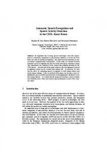
Fig. 1. The CHIL seminar room layout at the Universit¨ at Karlsruhe (TH).

and table-top microphones, where the problems are exacerbated by the much poorer quality of the acoustic signal. 2.1

Data Collection and Labeling

The data used for the experiments described in this work was collected during a series of seminars held by students and visitors at the Universität Karlsruhe (TH) in Karlsruhe, Germany, in the winter and early spring of 2004-2005. The seminar speakers spoke English, but usually with German or other European accents, and with varying degrees of fluency. This data collection was done in a very natural setting, as the students were far more concerned with the content of their seminars, their presentation in a foreign language and the questions from the audience than with the recordings themselves. Moreover, the seminar room is a common work space used by other students who are not seminar participants. Hence, there are many “real world” events heard in the recordings, such as door slams, printers, ventilation fans, typing, background chatter, and the like. The seminar speakers were recorded with a close-talking microphone (CTM) manufactured by Countryman Associates, a 64-channel Mark III microphone array developed at the US National Institute of Standards and Technologies (NIST) mounted on the wall, four T-shaped MAs with four elements mounted on the four walls of the seminar room and four Shure Microflex table-top microphones placed on a table in the center of the room. A schematic of the seminar room is given in Figure 1. All audio files were recorded at 44.1 kHz with 24 bits per sample. The high sample rate is preferable to permit more accurate position estimations, while the higher bit depth is necessary to accommodate the large

4


dynamic range of the far field speech data. Source localization and beamforming was performed on the “raw” 44.1 kHz data. For the purpose of ASR, the speech data was down-sampled to 16 kHz with 16 bits per sample after beamforming. In addition to the audio data capture, the seminars were simultaneously recorded with four calibrated video cameras that are placed at a height of 2.7 m in the room corners. Their joint field of view covers almost the entire room. The images are captured at a resolution of 640x480 pixels and a framerate of 15 frames per second, and stored as jpg-files for offline processing. The data from the CTM was manually segmented and transcribed. The data from the far distance microphones was labeled with speech and non-speech regions. The location of the centroid of the speaker’s head in the images from the four calibrated video cameras was manually marked every 0.7 second. Based on this marks the true position of the speaker’s head (ground truth) in three dimensions could be calculated within an accuracy of approximately 10 cm [3]. 2.2

Speaker Localization: Audio Features

The lecturer is the person that is normally speaking, therefore we can use audio features using multiple microphones to detect the speaker position. Consider the j-th pair of microphones, and let mj1 and mj2 respectively be the positions of the first and second microphones in the pair. Let x denote the position of the speaker in a three dimentional space. Then the time delay of arrival (TDOA) between the two microphones of the pair can be expressed as Tj (x) = T (mj1 , mj2 , x) =

kx − mj1 k − kx − mj2 k c

(1)

where c is the speed of sound. To estimate the TDOAs a variety of well-known techniques [4, 5] exist. Perhaps the most popular method is the phase transform (PHAT), which can be expressed as R12 (τ ) =

1 2π

Z

∞

−∞

X1 (ejωτ )X2∗ (ejωτ ) jωτ e dω |X1 (ejωτ )X2∗ (ejωτ )|

(2)

where X1 (ω) and X2 (ω) are the Fourier transforms of the signals of a microphone pair in a microphone array. Normally one would search for the highest peak in the resulting cross correlation to estimate the position. But since we are using a particle filter, as described in Section 2.4, we can simply set the PHAT value at the time delay position Tj (si ) of the MA pair j of a particular particle si as p(Aj |si ) = Rj (Tj (si ))

(3)

To get a better estimate we repeat this over all m pair of microphones (in our case 12), sum their values and normalize by m: m

p(A|si ) =

1 X p(Aj |si ) m j=1

(4)


5

Fig. 2. Snapshot from a lecture showing all 4 camera views (clockwise: camera 1,2,3,4). The native resolution is 640x480 pixels.

To get a (pseudo) probability value which tells us how likely this particle corresponds to a sound source we have to normalize over all values: p(A|si ) p(A|si ) = P i p(A|si )

(5)

As the values returned by the PHAT can be negative, but probability density function must be strictly nonnegative, we found that setting all negative values of the PHAT to zero yielded the best results. 2.3

Speaker Localization: Video Features

For the task of person tracking in video sequences, there is a variety of features to choose from. In our lecture scenario, the problem comprises both locating the lecturer and disambiguating the lecturer from the people in the audience. A snapshot from a lecture showing all 4 camera views is shown in Fig. 2. As lecturer and audience cannot be separated reliably by means of fixed spatial constraints as, e.g., a dedicated speaker area, we have to look for features that are more specific for the lecturer than for the audience. Intuitively, the lecturer is the person that is standing and moving (walking, gesticulating) most, while people from the audience are generally sitting and moving less. In order to exploit this specific behavior, we decided to use dynamic foreground segmentation based on adaptive background modeling as primary feature, a detailed explanation can be found in [6]. In order to support the track

6


indicated by foreground segments, we use detectors for face and upper body, also described in [6]. Both features (foreground F and detectors D) are linearly combined using a mixing weight β (for our experiments β was fixed to 0.7, this value was optimized on a development set), so that the particle weights for view j are given by p(V j |si ) = β · p(Dj |si ) + (1 − β) · p(F j |si )

(6)

To combine the different views, we sum over the weights from the v different cameras in order to obtain the total weight of the visual observation of the particular particle: v 1X p(V |si ) = p(V j |si ) (7) v j=1 To get a (pseudo) probability value which tells us how likely this particle corresponds to a vision source we have to normalize over all values: p(V |si ) p(V |si ) = P i p(V |si ) 2.4

(8)

Data Fusion with Particle Filter

Particle filters [7] represent a generally unknown probability density function by a set of random samples. Each of these particles is a vector in state space and is associated with an individual weight. The evolution of the particle set is a two-stage process which is guided by the observation and the motion model: 1. The prediction step: From the set of particles from the previous time instance, an equal number of new particles is generated. In order to generate a new particle, a particle of the old set is selected randomly in consideration of its weight, and then propagated by applying the motion model. In the simplest case, this can be additive Gaussian noise, but higher order motion models can also be used. 2. The measurement step: In this step, the weights of the new particles are adjusted with respect to the current observation. This means, the probability p(zt |xt ) of the observation zt needs to be computed, given that the state of particle xt is the true state of the system. As we want to track the lecturer’s head centroid, each particle si = (x, y, z) represents a coordinate in space. The ground plane is spanned by x and y, the height is represented by z. The particles are propagated by simple Gaussian diffusion, thus representing a coarse motion model: s0i = si · (Nσ=0.2m , Nσ=0.2m , Nσ=0.1m )

(9)

Using the features as described before in Sections 2.2 and 2.3, we can calculate a weight for each particle at time t by combining the probability of the acoustical observation At and the visual observation Vt using a weighting factor α: p(Pt |si ) = α · p(At |si ) + (1 − α) · p(Vt |si )

(10)


7

The weighting factor α was set by α=

m · 0.6 n

(11)

where n is the total number of microphone pairs and m the number of values above 0. The average value of α was approximately 0.4. Therefore, more weight was given to the video features. A particle’s weight is set to 0 if the particle leaves the lecture room1 or if its z-coordinate leaves the valid range for a standing person (1.2m < z < 2.1m). The final hypothesis about the lecturer’s location over the whole particle set 1 . . . m (in our case m = 300) can be derived by a weighted summation over the individual particle locations si,t at time t: m

Λt =

1X p(Pt |si ) · si,t i i

(12)

Sampled Projection Instead of Triangulation A common way to obtain the 3D position of an object from multiple views is to locate the object in each of the views and then to calculate the 3D position by using triangulation. This approach, however has several weak points: first of all, the object has to be detected in at least two different views at the same time. Second, the quality of triangulation depends on the points of the object’s images that are chosen as starting points for the lines-of-views: if they do not represent the same point of the physical object, there will be a high triangulation error. Furthermore, searching for the object in each of the views separately— without incorporating geometry information—results in an unnecessarily large search space. In prior work [8], we proposed using a variation of a Kalman filter to directly update the speaker position estimate based on the observed TDOAs. In particular, the TDOAs comprise the observation associated with an extended Kalman filter whose state corresponds to the speaker position. Hence, the new position estimate comes directly from the update formulae associated with the Kalman filter. In other work, we proposed an algorithm to incorporate detected face positions in different camera views into the Kalman filter without doing any triangulation. Our algorithm differs from that proposed by Strobel et al [9] in that no explicit position estimates are made by the individual sensors. Rather, as in the work of Welch and Bishop [10], the observations of the individual sensors are used to incrementally update the state of a Kalman filter. In the proposed method, we avoid the problems mentioned above by not using triangulation at all. Instead, we make use of the particle filter’s property to predict the object’s location as a well-distributed set of hypotheses: many particles cluster around likely object locations, and less particles populate the space in between. As the particle set represent a probability distribution of the 1

We restrict the particles to be within the full width of the room’s ground plane (0 < y < 7.1m) and half of the depth (0 < x < 3m).

8


predicted object’s location, we can use it to narrow down the search space. So instead of searching a neighborhood exhaustively, we only look for the object at the particles’ positions. When comparing the proposed method to Kalman Filter-based tracking, the following advantage becomes apparent: A particle filter is capable of modeling multi-modal distributions. In particular, this implies that no single measurement has to be provided and no information is lost by suppressing all but the strongest measurement, as is done by a Kalman filter. Moreover, no data association problem occurs as in the case when object candidates from different views must be matched in order to perform explicit triangulation. 2.5

Beamforming

In this work, we used a simple delay and sum beamformer implemented in the subband domain. Subband analysis and resynthesis was performed with a cosine modulated filter bank [11, §8]. In the complex subband domain, beamforming is equivalent to a simple inner product y(ωk ) = vH (ωk )X(ωk ) where ωk is the center frequency of the k th subband, X(ωk ) is the vector of subband inputs from all channels of the array, and y(ωk ) is the beamformed subband output. The speaker position comes into play through the array manifold vector [12, §2] vH (ωk ) = ejωk τ0 (X) ejωk τ1 (x) · · · ejωk τN −1 (x) where τi (x) = kx − mi k/s is the propagation delay for the h microphone located at mi . After beamforming, the subband samples are synthesized back into a time domain signal, and then downsampled to 16 kHz for ASR purposes. 2.6

Language Model Training

To train language models (LM) for LM interpolation we used corpora consisting of broadcast news (160M words), proceedings (17M words) of conferences such as ICSLP, Eurospeech, ICASSP or ASRU and talks (60k words) by the Translanguage English Database. Our final LM was generated by interpolating a 3-gram LM based on broadcast news and proceedings, a class based 5-gram LM based on broadcast news and proceedings and a 3-gram LM based on the talks. The perplexity is 144 and the vocabulary contains 25,000 words plus multi-words and pronunciation variants. 2.7

Acoustic Model Training

As relatively little supervised data is available for acoustic modeling of the recordings the acoustic model has been trained on Broadcast News [13] and merged with the close talking channel of meeting corpora [14] [15] summing up to a total of 300 hours of training material.


9

The speech data was sampled at 16kHz. Speech frames were calculated using a 10 ms Hamming window. For each frame, 13 Mel-Minimum Variance Distortionless Response (Mel-MVDR) cepstral coefficients were obtained through a discrete cosine transform from the Mel-MVDR spectral envelope [16]. Thereafter, linear discriminant analysis was used to reduce the utterance based cepstral mean normalized features plus 7 adjacent to a final feature number of 42. Our baseline model consisted of 300k Gaussians with diagonal covariances organized in 24k distributions over 6k codebooks. 2.8

Acoustic Adaptation: Close Talk Speech

The adaptation of the close talking acoustic model was done in consecutive steps: 1. A supervised Viterbi training of the CHIL adaptation speakers followed by a maximum a posteriori (MAP) combination of this model with the acoustic model of the original system: To find the best mixing weight, a grid search over different mixing weights was performed. The weight, which reached the best likelihood on the hypotheses of the first pass of the unadapted speech recognition system, was chosen as the final mixing weight. 2. A supervised maximum likelihood linear regression (MLLR) in combination with feature space adaptation (FSA) and vocal tract length normalization (VTLN) on the close talking CHIL development set: This step adapts to the speaking style of the lecturer and the channel. In the case of non-native speakers the adaptation should also help to cover some ’non nativeness’. 3. A second, now unsupervised MLLR, FSA and VTLN adaptation based on the hypothesis of the first recognition run: this procedure aims at adapting to the particular speaking style of a speaker and to changes within the channel. 2.9

Acoustic Adaptation: Far Distance Speech

The adaptation of the far distance acoustic model was done in consecutive steps: 1. Four iterations of Viterbi training on far distance data from NIST [17] and ICSI [18] over all channels on top of the acoustic trained models to better adjust the acoustic models to far distance. 2. A supervised MLLR in combination with FSA and VTLN on the far distance (single distance or MA processed) CHIL development set: This step adapts to the speaking style of the lecturer and the channel (in particular to the room reverberation). In the case of non-native speakers the adaptation should also help to cover some non-native speech. 3. A second, now unsupervised MLLR, FSA and VTLN adaptation based on the hypothesis of the first recognition run: this procedure aims at adapting to the particular speaking style of a speaker and to changes within the channel.

3

Experiments

In order to evaluate the performance of the described system, we ran experiments on recordings as described before on five seminars/speakers providing a total of approximately 130 minutes speech material with 16,395 words.

10

3.1


Source Localization

The error measure used for source localization is the average Euclidean distance between the hypothesized head coordinates and the labeled ones. Tracking mode Audio only Video only Video & Audio

Average error (cm) all frames speech frames 46.1 41.7 36.3 36.5 30.5 29.1

Table 1. Averaged error in 3D head position estimation of a lecturer over all frames (approx. 130 Minutes) and frames where speech was present (approx. 105 Minutes).

Based on the results reported in Table 1 we deduce that although the video only tracker performs considerably better than the audio only tracker, the performance can still be significantly increased by combining both modalities. This effect is particularly distinctive during one recording in which the lecturer is standing most of the time in one dark corner of the room, thus being hard to find using solely video features; the mean error for this seminar was 116 cm. While the video only tracker has the same performance for all frames and speech only frames, the precision of the audio only and the combined tracker is higher for the frames where speech is present compared to the precision over all frames. 3.2

Speech Recognition

The speech recognition experiments described below were conducted with the Janus Recognition Toolkit (JRTk), which was developed and is maintained jointly by the Interactive Systems Laboratories at the Universität Karlsruhe (TH), Germany and at the Carnegie Mellon University in Pittsburgh, USA. All tests used the language and acoustic models described above for decoding. Tracking mode Close Talking Microphone Microphone Array single microhone estimated position (Audio only) estimated position (Video only) estimated position (Audio & Video) labeled position

WER 34.0% 66.5% 59.8% 59.1% 58.4% 55.8%

Table 2. Word error rates (WER)s for a close talking microphone and a single microphone of the array and the microphone array with different position estimates.

As mentioned before, the main advantage offered by a MA is the relatively large reduction in WER over a single channel, as can be seen in comparing the

audio only

Average Error (cm)

40

video only Microphone Array Driven Speech Recognition

30

11

video & audio figures in Table 2. In fact, using a MA with an estimated speaker position over 20 far distance channel we gain back 26.9% of the accuracy compared to a single the CTM. labeled position 10 3.3 Effect of Source Localization Accuracy on ASR Figure0 3 compares the average position error of the source localization to the WER. If 55 the error the labeled position 56 of 57 58 59 60 to the ground truth is around 15 cm (our calculatinon of Error the accuracy is approximately 10 cm), then a linear Word Rate relationship can be seen.

audio only

Word Error Rate

60

video only

59 58

video & audio

57 56

labeled position

55 0

5

10

15 20 25 30 35 Average Error (cm)

40

45

Fig. 3. Plot comparing the average position error to the word error rate.

4

Conclusion

We have compared the WER on different approached for person tracking using multiple cameras and multiple pairs of microphones. The core of the tracking algorithm is a particle filter that works by estimating the 3D location by sampled projection, thus benefiting from each single view and microphone pair. The video features used for tracking are based on adaptive foreground segmentation and the response of detectors for upper body, frontal face and profile face. The audio features are based on the TDOA between pairs of microphones, and are estimated with a PHAT function. The tracker using audio and video input clearly outperforms both the audioand video-only tracker on the accuracy of the estimate resulting in a decrease of WER. One reason for this is that the video and audio features described in this paper complement one another well: the comparatively coarse foreground feature along with the audio feature guide the way for the face detector, which in turn gives very precise results as long as it searches around the true head position. Another reason for the benefit of the combination is that neither motion and

12


face detection nor acoustic source localization responds exclusively to the lecturer and not to people from the audience – so the combination of both increases the chance of actually tracking the lecturer and therefore a decrease in WER. In the future we want to use advanced techniques such as cepstral domain maximum likelihood beamformer [19] for the MA. For the fusion weight we want to define a criteria which depends on voice activity detection to give more weight to the audio in the case of speech and vice versa.

References 1. “Computers in the human interaction loop,” http://chil.server.de. 2. M. W¨ olfel and S. Burger, “The ISL baseline lecture transcription system for the TED corpus,” Submitted to Eurospeech, 2005. 3. D. Focken and R. Stiefelhagen, “Towards vision-based 3-d people tracking in a smart room,” IEEE Int. Conf. Multimodal Interfaces, 2002. 4. M. Omologo and P. Svaizer, “Acoustic event localization using a crosspowerspectrum phase based technique,” Proc. ICASSP, vol. II, pp. 273–6, 1994. 5. J. Chen, J. Benesty, and Y. A. Huang, “Robust time delay estimation exploiting redundancy among multiple microphones,” IEEE Trans. Speech Audio Proc., vol. 11, no. 6, pp. 549–57, November 2003. 6. K. Nickel, T. Gehrig, R. Stiefelhagen, and J. McDonough, “A joint particle filter for audiovisual speaker tracking,” Submitted to ICMI 2005, 2005. 7. M. Isard and A. Blake, “Condensation–conditional density propagation for visual tracking,” International Journal of Computer Vision, vol. 29, no. 1, pp. 5–28, 1998. 8. anonymous. 9. N. Strobel, S. Spors, and R. Rabenstein, “Joint audio-video signal processing for object localization and tracking,” in Microphone Arrays, M. Brandstein and D. Ward, Eds. Heidelberg, Germany: Springer Verlag, 2001, ch. 10. 10. G. Welch and G. Bishop, “SCAAT: Incremental tracking with incomplete information,” in Proc. Computer Graphics and Interactive Techniques, August 1997. 11. P. P. Vaidyanathan, Multirate Systems and Filter Banks. Englewood Cliffs: Prentice Hall, 1993. 12. H. L. Van Trees, Optimum Array Processing. New York: Wiley-Interscience, 2002. 13. Linguistic Data Consortium (LDC), “English broadcast news speech (Hub-4),” www.ldc.upenn.edu/Catalog/ LDC97S44.html. 14. F. Metze, C. F¨ ugen, Y. Pan, T. Schultz, and H. Yu, “The ISL rt-04s meeting transcription system,” in Proc. ICASSP-2004 Meeting RecognitionWorkshop. Montreal; Canada: NIST, 2004. 15. S. Burger, V. Maclaren, and H. Yu, “The isl meeting corpus: The impact of meeting type on speech style,” ICSLP, 2002. 16. M. W¨ olfel, J. McDonough, and A. Waibel, “Warping and scaling of the minimum variance distortionless response,” ASRU, 2003. 17. V. Stanford, C. Rochet, M. Michel, and J. Garofolo, “Beyond close-talk - issues in distant speech acquisition, conditioning classification, and recognition,” ICASSP 2004 Meeting Recognition Workshop. 18. A. Janin, J. Ang, S. Bhagat, R. Dhillon, J. Edwards, N. Morgan, B. Peskin, E. Shriberg, A. Stolcke, C. Wooters, and B. Wrede, “The icsi meeting project: Resources and research,” ICASSP 2004 Meeting Recognition Workshop. 19. D. Raub, J. McDonough, and M. W¨ olfel, “A cepstral domain maximum likelihood beamformer for speech recognition,” ICSLP, 2004.