Jul 1, 2009 - Keywords: migration motif, financial data mining, spatial- temporal pattern mining .... from financial data, undertake a detailed study of the US markets, and analyze the ...... A big jump across size is rare for motifs in these two ...
Migration Motif: A Spatial-Temporal Pattern Mining Approach for Financial Markets Xiaoxi Du†
Ruoming Jin†
Liang Ding‡
†
Department of Computer Science Kent State University, Kent, OH, 44242, USA
{xdu,jin,vlee}@cs.kent.edu ABSTRACT A recent study by two prominent finance researchers, Fama and French, introduces a new framework for studying risk vs. return: the migration of stocks across size-value portfolio space. Given the financial events of 2008, this first attempt to disentangle the relationships between migration behavior and stock returns is especially timely. Their work, however, derives results only for market segments, not individual companies, and only for one-year moves. Thus, we see a new challenge for financial data mining: how to capture and categorize the migration of individual companies, and how such behavior affects their returns. We propose a novel data mining approach to study the multi-year movement of individual companies. Specifically, we address the question: “How does one discover frequent migration patterns in the stock market?” We present a new trajectory mining algorithm to discover migration motifs in financial markets. Novel features of this algorithm are its handling of approximate pattern matching through a graph theoretical method, maximal clique identification, and incorporation of temporal and spatial constraints. We have performed a detailed study of the NASDAQ, NYSE, and AMEX stock markets, over a 43-year span. We successfully find migration motifs that confirm existing finance theories and other motifs that may lead to new financial models. Categories and Subject Descriptors: H.2.8 [Database Management]: Database Applications - Data Mining General Terms: Algorithms, Economics Keywords: migration motif, financial data mining, spatialtemporal pattern mining, trajectory mining, risk factor
1.
INTRODUCTION
The year 2008 witnessed the third worst performing stock market in more than one century and the start of the biggest economic recession in over 70 years. We are compelled to confront one of the most fundamental questions in financial and economic study: do we yet fully understand financial market risks? Over the past 40 years, a large body of financial literature has demonstrated that investment returns are driven by multiple factors, evolving from the
Permission to make digital or hard copies of all or part of this work for personal or classroom use is granted without fee provided that copies are not made or distributed for profit or commercial advantage and that copies bear this notice and the full citation on the first page. To copy otherwise, to republish, to post on servers or to redistribute to lists, requires prior specific permission and/or a fee. KDD’09, June 28–July 1, 2009, Paris, France. Copyright 2009 ACM 978-1-60558-495-9/09/06 ...$5.00.
Victor E. Lee†
John H. Thornton Jr.‡
‡
Department of Finance Kent State University, Kent, OH, 44242, USA
{lding,jthornt5}@kent.edu single market factor theory specified by the Capital Asset Pricing Model of Sharpe [18] and Lintner [15]. Each risk factor is said to have a premium, the average incremental return that the market awards investors for undertaking the additional risk. Perhaps the most commonly identified factors are those associated with the Fama and French three-factor model [5]: the size premium based on market value of equity and the value premium based on the price-to-book ratio (or other ratios comparing an accounting-based number to market value). Although controversial, many financial economists believe the size and value premiums to be important risk factors. However, existing financial analyses treat these factors as prior or static factors, and do not consider their changes. Indeed, the dynamics of these risk factors are largely unknown. To address this ignorance, Fama and French [7] recently investigated the dynamic nature of risk factors by examining movements of companies between portfolios based on size and the price-tobook ratio (P/B). They find that a significant portion of the value premium can by explained by the migration patterns of companies across portfolios. However, Fama and French examine migration patterns only from one year to the next. This raises the question as to whether there are multi-year patterns in the return data. Our paper attempts to answer this question by investigating multi-year migration patterns in a size-value grid. In data mining terms, the portfolio of each company corresponds to a moving trajectory over a two-dimensional financial grid (discretized size vs. discretized price-to-book ratio, a standard representation in financial circles). Thus, a migration pattern corresponds to a collection of subtrajectories which follow similar paths. This problem is related to sequential pattern mining [1], time series motif discovery [14, 19], and trajectory mining [13, 16, 10, 8], which have been extensively studied in data mining. However, the interesting properties of the financial market and its migration patterns distinguish our problem from these existing works and call for new mining techniques. First, financial data is noisy and may have estimated values, so financial migration motifs must make approximate rather than exact matches, requiring similarity functions unique to the application. Second, moving paths and migration motifs are meaningful only if they comply with both temporal (the timing of changes to the risk factors) and spatial (the degree of change) constraints. Specifically, the spatial constraints need to be represented in terms of the discrete financial grid, which is quite different from typical trajectory mining which focuses on Euclidean space. Third, each company typically stays at one financial grid point for a certain period of time and thus in their moving trajectory, each point is repeated many times. Applying current sequential pattern mining and motif discovery methods would likely generate many redundant (meaningless) patterns. How to handle such repetitions
is the key for effectively and efficiently extracting financially meaningful motifs. Interestingly, we find that this migration pattern mining problem is not unique to financial market study, but can also find applications in business and the social sciences. For instance, in customer relationship management (CRM), marketing researchers typically classify customers according to RFM: Recency (time of the last order), Frequency (quantity of orders), and Monetary value (value of orders). Further, to perform RFM analysis, each attribute is discretized to generate several categories [3] and thus produce a three-dimensional marketing grid. Current marketing practice utilizes such grids to analyze customer behavior and define market segments. However, how to categorize the dynamics of customer behavior, and how to adjust the managerial decision accordingly, remains on open problem in marketing. Thus, even though we focus on mining migration trajectories from financial data, our problem and algorithm can be easily generalized to similar problems in other domains.
which focuses on the discrete realm of categorical items and events. Trajectory mining and our problem target multivariate ordinal space and involve approximate matching in such space. Motif Discovery in Time Series: Several motif discovery approaches have been developed for time series data. Dynamic Time Warping [17] permits a limited amount of time or speed variation. Another avenue, usable for spatial variation as well, compares time series according to their Longest Common Subsequence [20]. LCSS has higher immunity to outliers [21], but it is not efficient for large sets of strings. Lin [14] uses a Monte Carlo projection method [2] to search randomly, reducing the expected time to find good matches. Recently, Minimum Description Length (MDL) has been applied to decompose time series and to identify interesting motifs [19]. Our problem and work differ from these works as we try to find motifs of any length, whereas these works focus on discovering motifs of a certain length. Also, our migration motif is specified by both spatial and temporal constraints, which are not included in other time series motif studies.
1.1
2.
Contributions
We develop new methodologies for mining migration trajectories from financial data, undertake a detailed study of the US markets, and analyze the results. Specifically, (1) we formalize the migration motif definition and its mining problem for company trajectories over the financial grid; (2) we develop an efficient mining algorithm by utilizing a compact trajectory pattern representation and a graph theoretical method, utilizing maximal cliques, to discover all migration motifs; (3) applying our tool to the financial data, we find interesting and significant motifs, not found in randomized data. Thus, these patterns are inherent and uniquely characterize the dynamics of the financial market. (4) We relate migration motifs to financial economic theory.
1.2
Related Work
Trajectory Mining: Trajectory mining has attracted much attention over the last several years due to the widespread use of location-acquisition technologies, such as GPS, GSM, sensor networks, and RFID. Researchers have developed methods for trajectory clustering, classification, and frequent pattern discovery [13, 16, 10, 8]. The existing work on trajectories focuses on physical geometric or geological space. Thus they aggressively utilize Euclidean space properties to define and approximate the trajectories [8, 13]. Since company trajectories move over the non-Euclidean financial grid, we cannot apply their similarity measures. Besides, most trajectory mining methods do not consider temporal factors, focusing only on the spatial properties of the moving path. In our problem, we must consider both spatial and temporal factors for the migration motifs. The trajectory pattern or simply T-pattern in [10] is very similar to our migration motif definition. The major contribution of their work is to identify region-of-interests, i.e., the discretized regions which are shared and visited by many trajectories. Then, they assign each region a unique symbol and apply the TAS (TemporallyAnnotated Sequence) algorithm (a frequent sequential pattern mining method) [9] to discover frequent patterns. What makes our problem unique is that each company is likely to stay at a location for a long time, and thus we have to deal with the repetition problem. Moreover, our migration motifs are defined in terms of pairwise-similar sub-trajectories, which is another difference from T-patterns. We also note that trajectory mining and our problem can be looked upon as a special case of sequential pattern mining [1],
PROBLEM DEFINITION
Our general goal is to find frequent patterns of company migration in size-value space. Following Fama and French [7], we consider two attributes of stocks in the US: market capitalization (size) and P/B ratio (value), forming a two-dimensional space. The stocks of firms with low P/B ratios are considered to be value stocks, while the stocks of firms with high P/B ratios are considered to be growth stocks. Fama and French partition the space into a 2 × 3 grid: {small, large} × {value, neutral, growth}. This grid size is too coarse to observe detailed migration patterns, so we increase the grid divisions to 10 × 10 and higher, setting boundaries by equally-sized percentiles ranges. We call this grid the Financial Grid. Company attributes are computed once per year. The location of each firm in the grid for year R is based on its size at the end of June that year and its P/B at the end of December of the previous year. That is, (x, y)r = (size(June(r)), value(Dec(r − 1)).
2.1
Trajectories and Sub-Trajectories
The Financial Trajectory of a company is simply a time sequence, denoted as (x1 , y1 ), (x2 , y2 ), · · · , (xn , yn ), where (xi , yi ) is the company’s ith discrete point (or location) in the financial grid G2 . Figure 1 shows an example of a financial grid and five trajectories, which will be used for a running example throughout this paper. The number next to each vertex is the duration that the company remains at that location.
Figure 1: Trajectories on a Financial Grid A Sub-trajectory is a subsequence of a trajectory. Formally, for a
given trajectory (x1 , y1 ), (x2 , y2 ), · · · , (xn , yn ), a sub-trajectory is a sequence (x′1 , y1′ ), (x′2 , y2′ ), · · · , (x′k , yk′ ), such that there exists 0 ≤ i1 < i2 < · · · < ik ≤ n, where (x′1 , y1′ ) = (xi1 , yi1 ), · · · , (x′k , yk′ ) = (xik , yik ). A sub-trajectory with k points is known as a k-length sub-trajectory. Note that a subtrajectory by itself describes neither the elapsed time nor the original path between its points. For this reason, we will sometimes refer to sub-trajectories as sub-trajectory patterns, since they embody more than one possible set of timings and detailed paths. However, not every sub-trajectory is of interest for financial analysis. We are only interested in those sub-trajectories satisfying certain temporal and spatial constraints. D EFINITION 1. (Sub-trajectory with Spatial and Temporal Constraints) The spatial constraint for a sub-trajectory requires the intermediate trajectory points (xk , yk ) between any two consecutive sub-trajectory points (xij , yij ) and (xij+1 , yij+1 ), ij ≤ k ≤ ij+1 , to be within a range defined by these two points. The temporal constraint for a sub-trajectory requires that the number of intermediate trajectory points between consecutive subtrajectory points be less than a limit U , that is, ij+1 − ij ≤ U . For instance, the simplest spatial range function requires intermediate points to be within the rectangular bounding box specified by the two consecutive sub-trajectory points, i.e., xij ≤ (≥)xk ≤ (≥)xij+1 and yij ≤ (≥)yk ≤ (≥)yij+1 , assuming xij ≤ (≥)xij+1 and yij ≤ (≥)yij+1 . The spatial constraint helps us to find the minimum number of descriptive points in a trajectory. The intermediate points need not be included because they are guaranteed to follow a bounded path from one sub-trajectory point to another. An upper bound time constaint is important in financial migration motif mining to model the short-term memory of investors. That is, even when long-term data is available for their consideration, investors tend to only consider a company’s recent history.
2.2
Migration Patterns and Motifs
We now consider the problem of finding similar sub-trajectories within a collection of trajectories. Let D be a set of financial trajectories {T1 , · · · TN }, where the time interval t is the same for all trajectories. (In our examples, t = 1 year.) Not every trajectory starts at the same absolute time, however. This problem could be simply converted into a sequential pattern mining problem by representing each grid point as a unique symbol. However, in financial data mining, exact sub-trajectory patterns may not capture the underlying behaviors shared by the companies due to noisy data. For example, book value is estimated and only available on a quarterly basis. Conversely, prices of publicly-traded stocks are available daily (even by the minute) but are very noisy. Hence, we are interested in a robustness measure for defining migration motifs. Specifically, we introduce the similarities (distance) between two (sub)trajectories. D EFINITION 2. (Distance between (Sub)Trajectories) For two aligned equal-length trajectories or sub-trajectories T = (x1 , y1 ), (x2 , y2 ), · · · , (xn , yn ) and T ′ = (x′1 , y1′ ), (x′2 , y2′ ), · · · , (x′n , yn′ ), their distance D(T, T ′ ) is the maximum of the distance between any two corresponding trajectory points: D(T, T ′ ) = max (d((xi , yi ), (x′i , yi′ ))) . In our study, the distance between two trajectory points is defined as the L1-norm (Manhattan distance), since we operate in discrete space. For example, in Figure 1, if we assume trajectories stay at a location for only one year, then
TW BC = (9, 5), (9, 2), (8, 3), (8, 1), (8, 3), (8, 1), (7, 2) TP U = (8, 1), (8, 3), (7, 1), (7, 3), (7, 1), (6, 1), (8, 1) D(TW BC , TP U ) = max(5, 2, 3, 3, 3, 2, 2) = 5 D EFINITION 3. (Migration Motif) Given a set of trajectories k D = {T1 , · · · TN }, Let PD be all k-length sub-trajectories from D k (satisfying the spatial and temporal constraints). Let M ⊆ PD be a subset of k-length sub-trajectories, such that the following properties hold: (1) (pair-wise similarity) for any two sub-trajectories m1 , m2 ∈ M , d(m1 , m2 ) ≤ ǫ; (2) (maximal) adding any other sub-trajectories to M will violate condition 1; (3) (frequent) the sub-trajectories in M come from at least θ different trajectories. That is, if C = the set of trajectories which cover M , then |C| ≥ θ. A set M of sub-trajectories satisfying these properties is a k-length sub-trajectory pattern or k − ǫ − θ-migration motif. Companies often stay at the same grid location for consecutive years. Such repetition can result in many redundant sub-trajectories from one company. Thus, requirement 3 for distinct trajectories prevents us from over-counting the effect of the repetition. It also helps to avoid over-counting the effect of a few trajectories which have cyclic behavior.
3.
ALGORITHMS
Given a support threshold θ and distance threshold ǫ, we would like to discover all the migration motifs. Our algorithm is built on two novel techniques: (1) a compact trajectory and pattern representation, which can significantly reduce the number of sub-trajectories, and (2) the combination of maximal clique and sequence-expanding properties. We will introduce these techniques in turn and then give the overall mining algorithm.
3.1
Compact Trajectory and Pattern Representation
As we mentioned before, financial trajectories are very special because a firm often stays at one gird location for a number of years. For instance, consider a trajectory which stays at one location for 10 years and then moves to another location for the next 10 years. If these two locations happen to belong to a migration motif and the time constraint U ≥ 10 years, then this small trajectory alone generates 100 valid sub-trajectories. An upper bound for Qthe number of sub-trajectories produced by a single trajectory is i min(ci , U ), P where ci is the time spent at location i, i ci = length of the trajectory. If U is very relaxed, we can have an exponential number of sub-trajectories. Additionally, we have to consider the spatial and temporal constraints for each sub-trajectory. This type of repetition makes the motif mining very challenging, considering we have to extract motifs from a vast number of sub-trajectories. To deal with these difficulties, we introduce a compact trajectory and pattern representation which significantly reduces the computational cost of pattern mining by combining overlapped patterns into a single object. In a trajectory (x1 , y1 ), (x2 , y2 ), · · · , (xn , yn ), if the company stays at the same location for consecutive time periods, we merge the consecutive points into one and record time spent. Thus, we have the following representation: (x′1 , y1′ ) : z1 , (x′2 , y2′ ) : z2 , · · · , (x′k , yk′ ) : zk , where for any i, (x′i , yi′ ) 6= ′ ). This representation not only reduces memory cost, (x′i+1 , yi+1 but most importantly, it reduces the enumeration cost. Given this, we introduce the embedding of a sub-trajectory pattern as follows. D EFINITION 4. (Sub-Trajectory Embedding) A sub-trajectory embedding is recorded in the following format: i1 :(x′i1 , yi′1 ):[s1 , e1 ],
second one considers how to build smaller-length trajectory embeddings into longer-length trajectory embeddings.
location
U=3 S1
S2
S3
Algorithm 1 EnumerateEmbedding2(Ti )
x1 1
2
3
4
1
2
3
4
x2 E U
U time
Figure 2: Timing Constraint on Subtrajectory Embedding · · · , ik :(x′ik , yi′k ):[sk , ek ], where each ij is an index of the corresponding location in the compact trajectory representation, i1 < i2 < · · · < ik , and [sj , ej ] is the range of valid time points for the corresponding location (1 ≤ sj ≤ ej ≤ zij ). We will apply the sub-trajectory embedding to effectively compress the sub-trajectory patterns. Note that such an embedding conQ tains a total of 1≤j≤k (ej −sj +1) possible sub-trajectory patterns of the original trajectory. It is easy to see that if one embedded pattern satisfies the spatial constraint, then the entire embedding satisfies the constraint, since member patterns describe the same location-sequence. This one-all property does not hold for the temporal constraint. Instead, for any tj in the range sj ≤ tj ≤ ej , there is at least one valid sub-trajectory appearing at that location at that time. Figure 2 illustrates how timing constraints on a sub-trajectory embedding. Since we need to show time on the horizontal axis, we represent location as a single dimension on the vertical axis. If U = 3, then we cannot include all 4 points from each location. Instead, we are limited to a range of 3 from the location transition. This gives us embedding 1:(x1 ):[2, 4], 2;(x2 ):[1, 3], represented by arrow E. The three multi-arrows S1 , S2 , S3 , each of length U , summarize the actual sub-trajectories contained within E. S1 contains the one valid sub-trajectory that can start as early as the 2nd time point of the first location. S2 starts one time point later and embodies two valid sub-trajectories. S3 starts at the last time point of the first location and includes U = 3 sub-trajectories. Note that E is the union of these three multi-arrows, but no single sub-trajectory can span the full range of E. Given this complication, how can we efficiency test whether an embedding satisfies the temporal constraint? The following lemma helps us solve this problem. L EMMA 1. For an index ij in a sub-trajectory embedding, let Z(ij ) be the absolute starting time for that interval in the original Pij −1 trajectory, i.e., Z(ij ) = k=1 zk . Then, for any two consecutive intervals in the sub-trajectory embedding, [sj , ej ] and [sj+1 , ej+1 ], the following two conditions suffice for validating the time constraint for a sub-trajectory embedding (U is the timing constraint threshold): Z(ij+1 ) + sj+1 − (Z(ij ) + sj ) ≤ U Z(ij+1 ) + ej+1 − (Z(ij ) + ej ) ≤ U Additionally, an embedding is maximal if any extension of its interval (increasing ej+1 or decreasing sj ) would produce a nonvalid embedding. The maximal property allows us to maximally compress the sub-trajectory patterns.
3.2
Efficiently Generating Embeddings
Now we consider two basic procedures for constructing the valid and maximal sub-trajectory embeddings. The first one addresses the base case, finding the 2-length trajectory embeddings, and the
Parameter: T rajectory Ti : (x′1 , y1′ ) : z1 , · · · , (x′k , yk′ ), U 1: R ← ∅ 2: for i = 1 to k − 1 do 3: t ← 0 {time difference from start to end} 4: Xmin ← x′i , Ymin ← yi′ ,Xmax ← x′i , Ymax ← yi′ {initialize bounding box} 5: for j = i + 1 to k do 6: if t < U {time constraint threshold} then 7: Xmin ← min(Xmin , x′j ) {update bounds} 8: Ymin ← min(Ymin , yj′ ) 9: Xmax ← max(Xmax , x′j ) 10: Ymax ← max(Ymax , yj′ ) 11: if (Xmin , Ymin ):(Xmax , Ymax ) ⊆ B((x′i , yi′ ):(x′j , yj′ )) {spatial constraint} then 12: s1 ← max(1, t + zi − U + 1) 13: e2 ← min(zj , U − t) 14: S ← i : (x′i , yi′ ) : [s1 , zi ] {first element} 15: E ← j : (x′j , yj′ ) : [1, e2 ] {second element} 16: R ← R ∪ (S, E) {add to the result set} 17: end if 18: t ← t + zj 19: end if 20: end for 21: end for 22: return R
Finding 2-Length Trajectory Embeddings: L EMMA 2. Algorithm 1 enumerates all the valid and maximal 2-length trajectory embeddings which satisfy both spatial and temporal constraints. If the timing and spatial constraints are very loose, this algorithm will generate k2 embeddings, for N trajectories of (average) length k. If the constraints are tight, the result size will be closer to N k. The time complexity is proportional to the result set size. To list each subtrajectory explicitly, without using the embedding format, would take O(N k2 U 2 ). Merging Sub-trajectory Embeddings: Here we consider how to merge a k-length and a 2-length sub-trajectory embedding (both from the same master trajectory) to form a k +1-length embedding. Let the two pre-merge sub-trajectory embeddings be as follows: T
=
i1 : (xi1 , yi1 ) : [s1 , e1 ], · · · , ik : (xik , yik ) : [sk , ek ]
′
=
j1 : (xj1 , yj1 ) : [s′1 , e′1 ], j2 : (xj2 , yj2 ) : [s′2 , e′2 ]
T
If the last index of T is the same as the first index of T ′ (ik = j1 ), we can merge them. However, due to the time constraint U , merging affects not only the time ranges of the overlap location, but also the ranges of the locations before and after it. We identify the following three timing rules. To distinguish the various embeddings, let the time ranges of the merged embedding be called [ai , bi ]. First, for the commonly shared location ik /j1 , the maximal time range is the overlap of the two input ranges. An overlap exists if ek ≥ s′1 . Then, [ak , bk ] = [sk , ek ] ∩ [s′1 , e′1 ] = [max(sk , s′1 ), min(ek , e′1 )]
(1)
We observe that if the time range for location i is set, then constraint U has a propagating effect on the locations before and after: bi+1 = f (bi ) and ai−1 = f (ai ). This is illustrated in Figure 3. Rule (2) addresses locations after the overlap point. Since we use a
T=1:(x1,y1):[2:4], 2:(x2,y2):[1:3] U
U
location
x1 x2 x3 U
U
T’=1:(x’1,y’1):[2:4], 2:(x’2,y’2):[1:3] U
U a2
b2
time
Figure 3: Sub-Trajectory Merging Example 2-length embedding, there is only one such point: [ak+1 , bk+1 ] = [s′2 , min(e′2 , Z(j1′ ) − Z(j2′ ) + bk + U )] (2) = [s′k , min(e′2 , −e′1 + bk + U )] There are k-1 points before (to the left) of the overlap point. The third rule should be applied for c = (k − 1) downto 1, or until [ai , bi ] is unchanged from [si , ei ]: [ac , bc ] = [max(sc , Z(ic+1 ) − Z(ic ) + ac+1 − U ), ec ] = [max(sc , ec + ac+1 − U ), ec ] (3) If any of the intervals are empty, then these two embedding cannot be combined. We refer to this operation as Combine(T, T ′ ). Figure 3 illustrates the merging method. We again let U = 3. T and T ′ are spatially mergeable because (x2 , y2 ) = (x′1 , y1′ ). We apply temporal merging as follows: (a2 , b2 ) = (max(1, 2), min(3, 4)) = (2, 3) (a1 , b1 ) = (max(2, 2 + 4 − 3), 4) = (3, 4) (a3 , b3 ) = (1, min(3, −4 + 3 + 3) = (1, 2) Therefore, the merged sub-trajectory embedding TM = 1:(x1 , y1 ):[3, 4], 2:(x2 , y2 ):[2, 3], 3:(x3 , y3 ):[1, 2] L EMMA 3. If the existing k-length embeddings are maximal, then the procedure either produces a valid and maximal k + 1length embedding or determines that the two are not mergeable.
3.3
A DFS Mining Procedure
Given the compact pattern representation, we now consider the overall mining algorithm. The key observation here is that we can speed up our mining process using the motif-join operation which combines two shorter motifs into one longer motif. Specifically, let Mk be a k-length migration motif, and let M2 be a 2-length motif. Motif-Join: The join between Mk and M2 is denoted as Mk ⊕ M2 = {Combine(T, T ′ )|T ∈ Mk , T ′ ∈ M2 , and, T and T ′ belong to the same company.} Simply speaking, for each pair of embeddings, one each from Mk and M2 , we only join those two embeddings which belong to the same trajectory and which overlap such that the last point for the k-embedding is the first point for the 2-embedding. The motif-join operator has an important property, referred to as the pairwise similarity preservation property, i.e., for any two sub-trajectories T1 and T2 in Mk ⊕ M2 , they satisfy the pairwise similarity condition, i.e., their distance d(T1 , T2 ) ≤ ǫ. Further, we can see the following lemma. L EMMA 4. If Mk+1 is a (k + 1)-length migration motif, then, there exists a k-length motif and a 2-length motif, such that Mk+1 = Mk ⊕ M2 . Thus, from this lemma and the pairwise similarity preservation property of the motif-join operator, we can derive the following DFS algorithm to discover all the migration motifs efficiently.
Maximal clique and 2-length migration motif: All migration motifs must satisfy a strict pairwise similarity measure. However, using Lemma 4 and the similarity preservation property of the motifjoin operator, we only need to test pairwise similarity for the original 2-length motifs. That is, only the 2-length migration motifs need to be constructed from scratch. Specifically, we construct the similarity graph to extract 2-length motifs. Let Pi2 be the set containing all the 2-length sub-trajectories (satisfying the spatial and temporal constraints) of trajectory Ti . We construct the 2-length sub-trajectory similarity graph as GS (V, E), where V is the set of all 2-length sub-trajectories, ∪Pi2 . An edge (u, v) exists if distance d(u, v) ≤ ǫ. This implies that GS is sparse, because the grid partitions limit the number of possible neighbors. Let C be a maximal clique (complete subgraph) in GS . If the clique C has sub-trajectories coming from at least θ different trajectories, then this maximal clique corresponds to a migration motif. We apply the maximal clique enumeration algorithm introduced in [12] to discover maximal cliques from the 2-length sub-trajectory similarity graph and choose those ones satisfying the frequency constraint as the 2-length motifs. Later in the experimental study, we found this is very efficient for our datasets. Algorithm 2 MigrationMotifMiner(D) Parameter: D = {T1 , T2 , · · · , TN }, ǫ, θ {Stage 1: Enumerate All 2-Length Sub-Trajectory Embeddings} 1: V ← ∅ 2: for each Ti ∈ D do 3: V ← V ∪ EnumerateEmbedding2(Ti ) 4: end for {(Stage 2: Construct Similarity Graph; Find 2-Length Motifs} 5: Construct Similarity Graph G2 from V 6: Motifs ← Maximal Cliques satisfying Frequency Constraint 7: Represent motifs by the centroid of each location 8: M2 ← List of Embeddings for Each Migration Motif {Stage 3: Use DFS to enumerate longer motifs} 9: for each m ∈ M2 do 10: DFSEnumeration(m) 11: end for Procedure DFSEnumeration(m) 1: E ← CandidateExtension(m, M2 ) {sub-trajectories of M2 whose startpoints are close to the endpoint of m} 2: for each e ∈ E do 3: m′ ← M otif − join(m, e) {Produce a k-length motif} 4: if F requency(m′ ) < θ {mimimum support level} then 5: continue; 6: end if 7: if CentroidIndex(m′ ) ∈ H {hash table of results} then 8: Compare m′ with motifs sharing the same centroid index 9: if m′ matches an existing motif Mprev then 10: Add any new embeddings in m′ to Mprev 11: else 12: H ← H ∪ m′ 13: DFSEnumeration(m′ ) 14: end if 15: end if 16: end for 17: clean the embedding list of m; return H
Algorithm Description: Algorithm 2 shows our 3-stage mining algorithm. Stage 1 lists all the 2-length sub-trajectory embeddings by Algorithm 1. Stage 2 discovers 2-length motifs using the aforementioned method (Lines 5 ∼ 8). Stage 3 uses DFS to efficiently generate all the longer motifs from the 2-Length motifs. We recursively mine the k-length migration motifs, when k > 2. For each 2-length motif in M2 , we call the recursive procedure DFSEnumeration for this purpose. First, we use the CandidateExten-
Figure 4: NYSE Motifs:(10g/U 3/ǫ1/θ10)
Figure 5: NYSE Motifs:(20g/U 3/ǫ1/θ10)
sion procedure to find all spatially appropriate 2-length migration motifs to extend migration motif m (Procedure line 1). Note that this reduces the search space by quickly pruning those 2-length motifs which cannot be joined with the current working motif m. Our rule compares the centroid of the last location of all sub-trajectories in m and the centroid of the first location of all sub-trajectories in the candidate 2-length motif. A 2-length motif can be combined with m only if d((xk , yk ), (x′1 , y1′ )) < 2 × ǫ. It is easy to see if this is not the case, the two sub-trajectories cannot be combined, or are not mergeable. This operation places all the possible candidate 2-length motifs to extend m in E. Then, for each extension candidate in E, we use the motif-join procedure to join the embedding list of two migration motifs to produce a (k + 1)-length motif (Procedure line 2 ∼ 3, m ⊕ e). We test whether each m ⊕ e satisfies the frequency constraint, saving only those whose patterns are sufficiently frequent (DFSEnumeration lines 4 ∼ 6). Each new discovered motif is indexed using its motif-centroid , which is the (rounded) average of each dimension (Procedure line 7) and try to store it in a hash table. However, the same motif might be produced more than once, as a result of different motif joins. To quickly test whether the new motif has been detected before, we first check if other motifs have the same motifcentroid using the hash table. If we find a match, we compare their embedding lists and see if they are indeed the same.
centile range. Following the financial industry’s practice of setting global definitions of “small” and “large,” we use the same partitions for all three markets. We tested each combination of the following parameter values: U = {3, 4, 5}, ǫ = {0, 1, 2}, θ = {10, 15, 20}, where U is the temporal constraint, ǫ is the spatial constraint, and θ is the minimum support level. We also tested the following grid partitionings: (10× 10), (20 × 20), (50 × 50), and (100 × 100). Our algorithm is very efficient. One combination of the parameter values can be tested in less than 2 and half minutes, using an Intel 3.2 GHz dual-core Xeon CPU with 4GB RAM. Tables 1, 2 and 3 summarize the number of motifs (M x corresponds to x-length migration motifs) detected for the NYSE, NASDAQ, and AMEX markets, respectively, under selected conditions. We use the following shorthand notation to indicate parameter settings: (g/U/ǫ/θ), i.e. (10g/U 3/ǫ1/θ10), where g is for the number of grid partitionings.
4.
EXPERIMENTAL RESULTS
We applied our algorithm to the financial market data from the Center for Research in Security Prices (CRSP) and Compustat databases for the period 1964 to 2007. We include ordinary shares (share code 10 or 11) but exclude financial companies (SIC code 6000-6999), American Depository Receipts, and closed-end funds. We also require that companies exist in the metrics for at least 10 years. Each company belongs to one of three stock exchanges: NYSE, NASDAQ, and AMEX. After this filtering, we have 1717 companies in NYSE, 2675 in NASDAQ, and 825 in AMEX. Following Fama and French’s approach, we define size to be stock price times number of share outstanding according to CRSP. Book value is set as total assets minus liabilities plus deferred taxes and investment tax credit, if available, minus liquidating, redemption, or carrying value, of preferred stock from Compustat. In general, NYSE companies are relatively large, while NASDAQ and AMEX companies tend to be smaller. Therefore, we search for motifs in each exchange separately. The grid is formed by partitioning each axis into equally-sized percentile ranges, updated each year. E.g., when we target a 10 × 10 grid, cell (1,2) contains companies in the [0 : 10) size percentile range and the [10 : 20) P/B per-
4.1
Motif Sensitivity to Parameters
In the existing Finance literature, researchers usually use a 2×3 grid or at most a 10×10 grid to analyze the financial markets. Our results show that the conventional grid sizes are not sufficient to analyze the migration of risk factors. We observed that motif discovery is sensitive to the grid scale. For the NYSE, the 10 × 10 grid generates the maximum number of motifs, for any combination of U and ǫ. Meanwhile, the optimal grid partitioning for NASDAQ and AMEX markets is 50 × 50. The reason is that a large portion of NASDAQ and AMEX trajectories are entirely contained within the lowest size decile. A 10×10 grid is reasonable for NYSE, since its company’s trajectories tend to make large movements. Markets with more concentrated trajectories, like NASDAQ and AMEX, need a finer partitioning. We show this zoom-in effect in Figures 4, 5, 6, and 7. The longest motifs tend to appear with larger U and ǫ. This is expected, because larger values imply looser spatial and temporal constraints.
4.2
Statistical Significance of Motifs
We compared occurrences of motifs in real financial data vs. randomized datasets. To generate random but plausible data, we took each company’s compact trajectory and then randomly shuffled the order of its location points. Using 100 randomized datasets, we searched for motifs across a cross section of input parameters. Our results are shown in Tables 1, 2 and 3. Two-length motifs are common in both randomized and real data, so they may not be meaningful. According to the Z-values, however, the frequency of longer motifs in real data is significant, not merely due to random activity.
Table 1: NYSE Real vs. Randomized Data: (10g/U 3/ǫ1/θ10); (20g/U 5/ǫ1/θ10); (50g/U 5/ǫ2/θ10); (100g/U 5/ǫ1/θ10) Grid Dim.
10 × 10
20 × 20
50 × 50
100 × 100
Motif
Real Data
M2 M3 M4 M5 M6 M2 M3 M4 M5 M2 M3 M4 M5 M2 M3 M4 M5
996 1681 361 60 2 1659 591 201 17 1558 937 187 16 555 69 16 3
Mean 882.67 134.32 7.59 0.34 0.02 470.82 27.46 1.64 0 251.59 44.34 2.39 0.02 103.3 4.89 0.13 0
Table 2: NASDAQ Real vs. (50g/U 3/ǫ1/θ10); (100g/U 3/ǫ1/θ10) Grid Dim
50 × 50
100 × 100
Motif
Real Data
M2 M3 M4 M5 M6 M2 M3 M4 M5 M6
758 441 109 19 2 288 251 48 9 1
Mean 359.31 37.83 2.93 0.63 0 203.59 20.26 7.02 0.6 0.01
Randomized Std Dev Z-value 1031.88 0.11 158.01 9.79 10.53 33.55 1.033 57.77 0.14 14.22 404.72 2.94 25.32 22.25 2.53 78.77 0 0 186.53 7.00 40.57 22.00 4.67 39.54 0.20 80.51 74.21 6.09 4.32 14.84 0.38 41.73 0 0
Randomized Randomized Std Dev Z-value 305.80 1.30 32.98 12.22 3.78 28.08 1.30 14.20 0 0 144.71 0.58 15.79 14.62 6.65 6.16 1.36 6.19 0.10 9.98
Max 2880 482 46 5 1 1199 102 13 0 658 196 30 2 236 17 2 0
5.1
Grid Dim
10 × 10
20 × 20
50 × 50
100 × 100
Data: Max 875 111 17 6 0 451 68 33 8 1
These results show that risk factor migration in the stock market is not random, and should not be neglected. Companies show high frequent risk migration patterns, which implies that the return that compensates for risk may also be associated with a certain patterns. The risk migration patterns may possibly explain some market anomalies that cannot be fully explained with conventional asset pricing models.
5.
Table 3: AMEX Real vs. Randomized Data: (10g/U 3/ǫ1/θ10); (20g/U 3/ǫ1/θ10); (50g/U 3/ǫ2/θ10); (100g/U 4/ǫ1/θ10)
ANALYSIS AND DISCUSSION Motif Patterns
Figures 4 and 5 depict representative NYSE motifs. Likewise, Figure 6 shows ones for NASDAQ and Figure 7 for AMEX. Note that in the NASDAQ and AMEX figures, we have focused on certain size and P/B values to magnify the motifs. An interesting class of motifs shows an oscillating migration pattern, with a pronounced back and forth change of value or size, e.g., M5-58 in Figure 4 and M3-172 in Figure 6. We call this the oscillation migration. Fama and French [6] identify a convergence pattern using a short 1-year horizon. Our results imply that what Fama and French found is part of a longer horizon oscillation pattern. When the movement is horizontal (value oscillation), companies migrate back and forth between the P/B spectrums of value and growth stocks. In terms of stock returns, this migration pattern means shifting between the high average to low average market expected returns. The motifs we found strongly suggest that given a certain size, a company shows a consistent oscillation movement among the P/B cells. Our algorithm allows us to track such movement over a long horizon. The maximum length motif we found is M8 in NYSE (10g/U 4/ǫ2). Oscillation motifs can be explained economically by an argument similar to that advanced by Fama and
Motif
Real Data
M2 M3 M4 M5 M2 M3 M4 M5 M2 M3 M4 M5 M6 M2 M3 M4 M5 M6 M7
23 55 42 2 191 182 65 4 336 184 44 11 2 179 65 51 32 5 1
Mean 10.08 18.3 2.03 0.0 127.1 51.22 1.45 0 172.49 45.46 5.48 0.19 0.03 93.04 19.77 7.63 0.42 0 0
Randomized Std Dev Z-value 14.78 0.87 32.77 1.12 7.42 5.39 0.22 8.93 115.64 0.55 45.04 2.90 1.80 35.33 0 0 130.52 1.25 34.57 4.01 4.82 8.00 0.58 18.65 0.22 8.93 67.38 1.28 15.27 2.97 6.90 6.28 0.80 39.62 0 0 0 0
Max 72 190 49 2 374 155 7 0 409 123 20 4 2 212 60 30 4 0 0
French. Market power could erode the high profitability of growth companies, while P/B of value stocks tends to rise as companies restructure and improve in profitability. So, over several years we see a shifting back and forth along the P/B spectrum. Other possible explanations could be exogenous, such as investors’ irrational response or endogenous, such as the company’s life cycle. We find size oscillation to be much rarer than value oscillation. Some examples are M5-37 in Figure 4, M5-13 and M5-10 in Figure 5, and M5-3 in Figure 6. For size oscillation motifs, the P/B ratio of the companies usually is small, so those companies are value stocks. As Fama and French argued, value stocks have the potential to restructure so that it is possible for them to change their size very quickly.
5.2
Distribution of Motifs
The motifs, especially the longer motifs, are concentrated in certain areas in the size-value grid. We identify those areas by showing some highly representative motifs in different markets in Figures 4, 5, 6 and 7. In NYSE, the motifs tend to appear more frequently in the upper size range, e.g., M6-1 and M5-58 in Figure 4, and M4-184, M4-186, M5-16, and M6-2 in Figure 5. The members of these motifs are among the largest companies in the markets, such as General Motors (GM) in M5-58 in Figure 4. This implies that, once companies reach a very large size, their operation is relatively stable and predictable. The migration patterns of these large firms are probably due to cyclical macroeconomic factors. On the contrary, small companies may be more likely to bring unexpected and surprising performance (in terms of risk migration, jumping). Therefore, investors require a so-called “size premium” for them. However, most motifs for NASDAQ and AMEX appear in the smaller size range of the grid, e.g., M6-2, M5-17 in Figure 6 and M4-3 and M4-5 in Figure 7(c). A big jump across size is rare for motifs in these two markets. However, these two markets do show value oscillation motifs very similar to those of NYSE. The low P/B range is another area where motifs appear frequently. The size oscillation migration patterns are common in this area for all three markets, e.g., M5-37 in Figure 4, M5-10 in Figure 5, M5-3 in Figure 6, and M6-1 in Figure 7(d). The vertical oscillations imply the potential restructuring behaviors for value stocks. In addition, the market participants generally expect companies with high P/B to grow in size. We also capture this belief in M3-170 in Figure 6.
Average Starting Year
25 20 15 10 5 0
2
3
4
5
6
NYSE10×10
2
3
4
5
6
NASDAQ50×50
2
3
4
5
6
AMEX50×50
Motifs by Length and by Market
Figure 8: Company Age at Motif Start
Figure 6: NASDAQ Motifs:(50g/U 3/ǫ1/θ10)
Figure 7: AMEX Motifs: (10g/U 3/ǫ1/θ10); (20g/U 3/ǫ1/θ10); (50g/U 3/ǫ2/θ10); (100g/U 4/ǫ1/θ10)
5.3
Motif Timing
Company Life Cycle. We wish to see what migration motifs have to say about the life cycles of companies. We record a starting age for each company, the point at which its migration pattern is first captured by a motif. E.g., HESS CORP(HES) becomes the member of M6-1 after it exists in our dataset for 24 years (Age 24). Some companies may have come into existence prior to their listing in our dataset. Nevertheless, our measurement at least obtains a minimum age (lower bound). We then calculate the average starting age for all motifs of the same length, for NYSE (10g/U 3/ǫ1/θ10), NASDAQ (50g/U 3/ǫ1/θ10), and AMEX (50g/U 3/ǫ2/θ10). The mean with 1σ error bars are reported in Figure 8. These data show that, in general, companies appear in a migration pattern when they have at least several years of maturity. In other words, companies need to be “old” to show a more consistent migration path. The average age to show M3 and longer motifs in NYSE ranges from 12-18 years. Though NASDAQ and AMEX companies tend to be younger overall, they still need 6-8 years before the companies show a motif. This finding can be explained by the life cycle of companies. If a company survives in the capital market, it will generally grow to a large size, and the managerial operation tends to mature and be relative stable. For these companies the cyclical nature of the overall economy may drive the observed migration patterns. Average Staying Time. Our tests may provide an explanation for two famous finance anomalies, long-term return reversals (De Bondt and Thaler [4]) and short-term momentum (Jegadeesh and Titman [11]). De Bondt and Thaler [4] establish two portfolios, losers and win-
ners, based on historical performance. Losers are stocks that have had poor return over the past three years, and winners are those that had high returns over a similar period. They find that losers have much higher average returns than winners over the three years after the establishment of the portfolios. If we reevaluate De Bondt and Thaler’s finding with the migration approach, the winners portfolio will contain some value stocks located in the low end of the P/B spectrum, while the losers portfolio will contain some growth stocks located in the high end. In De Bondt and Thaler’s approach, winner and loser companies will tend to move to the opposite end of the return spectrum; in other words, opposite P/B ends from the migration perspective. We identify a few sample motifs with such characteristic. E.g., M5-58 in NYSE (10g/U 3/ǫ1/θ10). We record the average time spent in each cell before moving to another cell (staying time). M5-58’s companies’ staying time in (10, 1) is 1.9 years, which is about the time to name them winners, according to De Bondt and Thaler’s approach. But after being chosen as the winners, it is about time for those companies to migrate to the lower return range (10, 6), where they are likely to stay for 2-3 years, the period over which Debondt and Thaler calculate their abnormal return. This migration pattern provides a reasonable explanation for reversal of the winner portfolio in their tests. In addition, our tests find that loser portfolios, which are on the left side of our financial grid, are likely to migrate after 2-3 years (e.g., in M5-58 from (10,8) to (10,1)), from the lower return range to the higher return range. This is the loser reversal of De Bondt and Thaler. Jegadeesh and Titman [11] find that strategies which buy stocks that have performed well in the past and sell stocks that have performed poorly in the past generate significant positive returns over 3 to 12 month holding periods. Our results show that stocks’ average staying time is longer than one year. This means that risk migration is lower frequency than momentum strategy’s turnover period. This could imply that momentum is caused either by the unchanged risk factors or by other risk factors that migrate in high frequency. Overall, our tests show that migration is a common phenomenon for the listed companies. Unlike other recent studies in migration [7, 6], our tests provide a quantitative approach to describe the long-term historical migration path for companies. Motif Relation to Calendar Years. We list the membership information for several typical motifs in NYSE and NASDAQ (Table 4). For each motif, we provide each company’s ticker and time span. For motifs with value oscillation paths, members’ time spans are highly concentrated. For example, in NYSE, in M5-45, all members join the motif from 1982-1984 and leave it from 1988-1991. This tight time span is characteristic of all the representative motifs we identified in Figures 4 and 6. The motifs with significant jumps show a slightly different pattern. E.g., M6-1 in NYSE and M3-22 in NASDAQ have starting years in the ranges 1966-1984 and 1976-2003. Although the years
Table 4: Motif Company Time Span Motif N Y S E 10 × 10 N A S D A Q 50 × 50
M5-45
M6-1
M3-22
M3-172
M4-50
Ticker[Time Span] IALU[’82-’91],ESX[’82-’88],CEM[’83-’88] SCX[’83-’89],CRI[’83-’91],NICO[’84-’88] RTS[’84-’88],EDE[’84-’91],OCQ[’84-’91] TOK[’84-’90], JM[’66-’72],CUE[’66-’73],ANR[’66-’74] PD[’67-’75],ZB[’67-’75],MRO[’84-’93] HES[’94-’02],CEG[’94-’02],PGN[’94-’06] AEE[’94-’06] ECOA[’77-’85],HELE[’78-’83],KUST[’76-’86] TRNS[’02-’06],SATC[’03-’05],TGAL[’03-’06] CRPB[’91-’94],SPSI[’92-’94],SMTH[’94-’97] CMED[’93-’95] ATTC[’88-’90],AWST[’88-’90],CHTT[’88-’90] IINT[’88-’90],NRRD[’88-’90],SHEL[’88-’90] ISO[’88-’90],ROPK[’88-’90],DTSI[’88-’90] FARC[’88-’90],WMSI[’88-’90],BPMI[’88-’90] NOLD[’74-’80],BFLD[’77-’81],UESC[’80-’84] UTRK[’84-’88],BRDL[’90-’93],NEWP[’92-’95] RDGE[’92-’96],IICR[’94-’97],STCIA[’95-’99] IMKTA[’00-’04],HGGR[’97-’04]
are widely spread, we can classify them into several periods. For M6-1, JM, CUE, ZB, PD, and ANR start in 1966-1967; HES, CEG, PGN, AEE in 1994, and MRO in 1984. For M3-22, ECOA, HELE, and KUST start in 1976-1978; MED, CRPB, SPSI, SMTH in 19911994, and TRNS, SATC, TGAL in 2002-2003. In contrast, there is no clear clustering of starting years for vertical oscillation motifs. E.g., M5-37 in NYSE ranges from 19652002, and M5-3 and M4-50 in NASDAQ range from 1974-2000. The causes for synchronicity (and asynchronicity) of motifs are not fully known. One possible explanation could be industry effect, that companies in the same industry may tend to move at the same period. However, our results do not support the hypothesis. Although we find some companies in some motifs come from the same industry, for most motifs, the membership is widely spread in different industries. For example, even for NASDAQ, a market with highly concentrated industries, no company in M5-17 comes from the same industry. We believe there exist market-level factors to cause the clustering of starting years, although there is no conclusive analysis on these factors. Market interest rate could be part of the cause. When the market interest rate moves, the market value and the book value of companies in general will change in the same direction. However, each company’s sensitivity of market value and book value to the market interest rate is different. This may bring different changes in P/B ratios. All this may cause some companies to appear in the same value oscillation pattern in the same period. If this is the case, then investors should pay more attention to market-level risk factors, e.g., interest rate, to evaluate the company risk migration. However, this explanation is not conclusive. We believe further research is needed to identify the cause of the migration patterns and their characteristics.
6.
CONCLUSION
We have developed an efficient and novel method to discover migration motifs in a financial grid, using a graph theoretical approach for performing approximate matching and incorporating spatial and temporal constraints. To our knowledge our study is the first attempt to find multi-year migration patterns in a financial dataset. Our also extends the work of Fama and French [7], which studies migration patterns over a one year time horizon. Perhaps the most interesting finding from our study is the existence of long hori-
zon oscillation patterns in the financial data. Our method detects motifs in which firms migrate back and forth between “value” and “growth”. This oscillation pattern may help to explain the so called “value premium” identified by past financial researchers. This pattern may also help to explain the long term mean reversion of stock returns found in De Bondt and Thaler [4]. We see opportunities to apply our algorithm to conduct further experiments to study financial hypotheses. For example, it may be possible to identify firms that have a high probability of entering an oscillating pattern. If successful, such an exercise could provide investors a signal as to which stocks are likely to have high (or low) returns over the next few years.
7.
REFERENCES
[1] Rakesh Agrawal and Ramakrishnan Srikant. Mining sequential patterns. In Proc. ICDE’95, pages 3–14, 1995. [2] J. Buhler. Efficient large-scale sequence comparison by locality-sensitive hashing. Bioinformatics, 17(5):419–428, 2001. [3] G. J. Cullinan. Picking them by their batting averages: recency-frequency-monetary method of controlling circulation. Manual release 2013, 1977. [4] Werner F. M. De Bondt and Richard Thaler. Does the stock market overreact? J. Finan., 40(3):793–805, 1985. [5] Eugene F. Fama and Kenneth R. French. Common risk factors in the returns on stocks and bonds. J. Finan. Econ., 33(1):3–56, Feb 1993. [6] Eugene F. Fama and Kenneth R. French. The anatomy of value and growth stock returns. Finan. Analysts J., 63(6):44–54, 2007. [7] Eugene F. Fama and Kenneth R. French. Migration. Finan. Analysts J., 40:48–58, 2007. [8] Scott Gaffney and Padhraic Smyth. Trajectory clustering with mixtures of regression models. In Proc. KDD’99, pages 63–72, 1999. [9] Fosca Giannotti, Mirco Nanni, and Dino Pedreschi. Efficient mining of temporally annotated sequences. In Proc. SDM’06, pages 346–357, 2006. [10] Fosca Giannotti, Mirco Nanni, Fabio Pinelli, and Dino Pedreschi. Trajectory pattern mining. In Proc. KDD’07, pages 330–339, 2007. [11] Narasimhan Jegadeesh and Sheridan Titman. Returns to buying winners and selling losers: Implications for stock market efficiency. J. Finan., 48(1):65–91, 1993. [12] Ina Koch. Enumerating all connected maximal common subgraphs in two graphs. Theor. Comput. Sci., 250(1-2):1–30, 2001. [13] Jae-Gil Lee, Jiawei Han, and Kyu-Young Whang. Trajectory clustering: a partition-and-group framework. In Proc. SIGMOD’07, pages 593–604, 2007. [14] Jessica Lin, Eamonn Keogh, Stefano Lonardi, and Pranav Patel. Finding motifs in time series. In Proc. 2nd Workshop on Temporal Data Mining, pages 53–68, 2002. [15] John Lintner. The valuation of risk assets and the selection of risky investments in stock portfolios and capital budgets: A comment. Rev. Econ. & Stat., 47(2):13–37, 1965. [16] Yunhao Liu, Lei Chen, Jian Pei, Qiuxia Chen, and Yiyang Zhao. Mining frequent trajectory patterns for activity monitoring using radio frequency tag arrays. In Proc. PerCom’07, pages 37–46, 2007. [17] H. Sakoe and S. Chiba. Dynamic programming algorithm optimization for spoken word recognition. IEEE Trans. Acoustics, Speech, and Signal Processing, 26(1), 1978. [18] William F. Sharpe. Capital asset prices: A theory of market equilibrium under conditions of risk. J. Finan., 19(3):425–442, 1964. [19] Yoshiki Tanaka, Kazuhisa Iwamoto, and Kuniaki Uehara. Discovery of time-series motif from multi-dimensional data based on mdl principle. Mach. Learn., 58(2-3):269–300, 2005. [20] Michail Vlachos, Dimitrios Gunopoulos, and George Kollios. Discovering similar multidimensional trajectories. In Proc. ICDE’02, page 673. IEEE Comput. Soc., 2002. [21] Michail Vlachos, Dimitrios Gunopulos, and George Kollios. Robust similarity measures for mobile object trajectories. In Proc. DEXA Workshops, pages 721–728. IEEE Comput. Soc., 2002.