Minimum Variance Modulation Filter for Robust Speech Recognition

MINIMUM VARIANCE MODULATION FILTER FOR ROBUST SPEECH RECOGNITION Yu-Hsiang Bosco Chiu and Richard M Stern Department of Electrical and Computer Engineering and Language Technologies Institute Carnegie Mellon University, Pittsburgh PA 15213 USA {ychiu,rms}@cs.cmu.edu ABSTRACT This paper describes a way of designing modulation filter by datadriven analysis which improves the performance of automatic speech recognition systems that operate in real environments. The filter for each nonlinear channel output is obtained by a constrained optimization process which jointly minimizes the environmental distortion as well as the distortion caused by the filter itself. Recognition accuracy is measured using the CMU SPHINX-III speech recognition system, and the DARPA Resource Management and Wall Street Journal speech corpus for training and testing. It is shown that feature extraction followed by modulation filtering provides better performance than traditional MFCC processing under different types of background noise and reverberation. Index Terms— filter design, automatic speech recognition, modulation frequency analysis, data analysis 1. INTRODUCTION Although feature extraction for automatic speech recognition (ASR) using conventional Mel-frequency cepstral coefficients (MFCC) [1] and perceptual linear prediction (PLP) [2] performs reasonably well when acoustical conditions for training and testing are matched, recognition accuracy degrades significantly when training and testing conditions are mismatched as in noisy or reverberant environments. Motivated by experimental observations that the neuronal response of mammalian auditory cortex is tuned to lower temporal modulation rates (e.g. [3]), and that humans are most sensitive to modulation frequencies in the range of 4 to 16 Hz (e.g. [4, 5]), a number of feature extraction methods have been proposed in recent years that exploit temporal information. These systems typically provide a recognition accuracy that exceeds that obtained using MFCC or PLP features in the presence of noise and other adverse conditions [6, 7, 8], especially if they are combined with a traditional recognition system in some fashion. In this paper, we first introduce the possibility of applying a linear-phase filter obtained from modulation frequency analysis for extracting robust features. We then present a data-driven strategy that can be used to design such filter set on a sentence-by-sentence basis. In Sec. 2 we review some of the previous work that has motivated our filter formulation and system implementation, and we describe feature processing method that we propose. Finally in Sec. 3, we evaluate the performance of our processing in several different types of noisy and reverberant environments. 2. MODULATION FREQUENCY ANALYSIS Modulation frequency components in speech signals have long been believed to be important in human recognition of speech. For exam-

ple, by assessing the change of modulation index under environmental distortion, Steeneken and Houtgast proposed a Speech Transmission Index (STI) which is highly correlated with subjective scores under different distortions [9]. In addition, by studying the contribution of different modulation frequency bands to automatic speech recognition accuracy, Kanedera et al. concluded that modulation frequency components in the range of 1 to 16 Hz contribute the most to ASR accuracy [10]. Inspired by these results, we focus in this paper on the design of a filter that operates in the modulation domain with three objectives in mind. First, as different sentences could be subjected to different types of distortion, we want our modulation filter to be data driven, so that the filter’s frequency response would be appropriate to different environmental conditions. Second, we define the environmental distortion whose effect on speech signals our filter attempts to minimize as the change of the modulation frequency components of the power spectrum. Finally, the filter itself should cause as little distortion as possible when the input signal is close to that of clean speech. 2.1. Filter design by modulation frequency analysis With the three objectives mentioned above in mind, we obtain the filter that minimizes the statistic Z π Z π ρ = λ |H(ω)|2 PN (ω)dω + |1 − H(ω)|2 PS (ω)dω (1) −π

−π

where λ is a free parameter that controls the balance between the degree of minimization of distortion caused by the environment (PN (ω)) and the distortion of the original modulation spectrum caused by the filter: |MS (ω) − MS (ω)H(ω)|2 = |1 − H(ω)|2 |MS (ω)|2 = |1 − H(ω)|2 PS (ω)

(2)

where MS (ω) is the modulation spectrum, obtained by computing the Fourier transform of each nonlinear channel output of clean speech utterance. Note that both phase and magnitude are considered. The frequency response of the filter is of the form (L−1)/2

H(ω) =

X

h(l)e−jωl

(3)

l=−(L−1)/2

We assume that a Type I linear phase filter with L odd and h(l) = h(−l) can be utilized to achieve our goal, without providing any further constraints on its frequency response at the outset. The expression that minimizes ρ can also be expressed as

2.2. System implementation L−1 Z π L−1 2 2 X X −jωk h(k)e )( h(l)∗ ejωl )PN (ω)dω ρ=λ (

−π k=− L−1 2

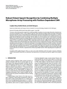
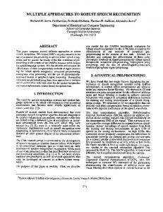
We apply the filter described above to the output of each channel of the system shown in Fig. 1, which is based on the system proposed by Chiu and Stern [11]. After windowing the incoming signal into frames of brief duration, a short-time Fourier Transform is applied to obtain the magnitude spectrum of each frame. Each frequency component is weighted by the weighting function shown in Fig. 2 to account for the equal loudness curve in the human auditory system [12]. After applying the triangularly-shaped Mel-scale filter with log compression, a logistic function is introduced to model the nonlinear function that relates the observed average auditory-nerve response as a function of the input level in decibels. α xi (m) = (10) 1 + exp(w1 ·yi (m) + w0 )

l=− L−1 2

L−1 L−1 Z π 2 2 X X + (1− h(k)e−jωk )(1− h(l)∗ ejωl )PS (ω)dω

−π

k=− L−1 2

=λ

l=− L−1 2

L−1 2

L−1 2

X

X

Z π h(k)h(l)∗ PN (ω)ejω(l−k) dω −π

k=− L−1 l=− L−1 2 2 L−1 2

L−1

Z π Z π 2 X X h(k) PS (ω)e−jωk dω− h(l)∗ PS (ω)ejωl dω − −π

k=− L−1 2

+

L−1 2

L−1 2

X

X

l=− L−1 2 π

Z

h(k)h(l)

k=− L−1 l=− L−1 2 2

∗

jω(l−k)

PS (ω)e −π

−π

Z π dω+ PS (ω)dω −π

Z π = λhT RN h − 2hT rS + hT RS h + PS (ω)dω

(4)

−π 1 3 rS ( L− ) 2 : 6 7 6 7 where rS =6 rS (0) 7, rS (k) = rS (−k) assuming that h is real. 4 5 : L−1 rS ( 2 ) The matrices RN and RS represent the autocorrelation matrices of the distortion and speech components, respectively, of the inputs to the filter H(ω). If we further assume that the distortion and speech modulation frequency components are uncorrelated, i.e. RN +S = RN + RS , the above equation can also be written as: Z π ρ = λhT(RN +S −RS )h+hTRS h−2hTrS + PS (ω)dω −π Z π T T T = λh RN +S h+(1−λ)h RS h−2h rS + PS (ω)dω (5)

2

where the coefficients α = 0.05, w0 = 0.613, w1 = −0.521 were determined empirically by evaluation using the Resource Management development set in additive white noise at 10 dB. These values are used in all our experiments. yi (m) is the log of the output of the ith channel. After the rate-level nonlinearity, the autocorrelation matrix elements rS (k) and rN +S (k) are estimated according to Eqs. (8) and (9) to obtain the coefficients of the filter in each channel through which the outputs of the nonlinearities are passed. R

log signal

h = (λRN +S + (1 − λ)RS )−1 rS

(7)

In the expression above, the (i, j)th element of the L×L autocorrelation matrix incoming noisy speech RN +S is denoted by rN +S (i − j), and the corresponding element of the L×L Toeplitz autocorrelation matrix RS obtained from the clean speech used to train the system is rS (k). The elements rS (k) and rN +S (k) are obtained by: C M i −k X X 1 xS (m)xS (m + k) i=1 (Mi − k) i=1 m=1

rS (k) = PC rN +S (k) =

1 M −k

M −k X

xN +S (m)xN +S (m + k)

(8)

(9)

m=1

where C is the number of training utterances and Mi is the number of frames of each training utterance and M is the number of frames of the incoming utterance. The observations xS (m) and xS+N (m) are the inputs to H(ω) in each channel (with mean subtraction) when the system inputs are clean and noisy speech, respectively.

log |FFT| …

…

fil …

D CT

… R

log

fil

Fig. 1. Block diagram of the feature extraction system. 5

−π

0 −5

gain (dB)

Taking the derivative with respect to h and setting it equal to zero we obtain ∂ρ = 2λRN +S h + 2(1 − λ)RS h − 2rS = 0 (6) ∂h producing the filter coefficients

fil R

−10 −15 −20 −25 −30 −35 0

2000

4000

6000

8000

frequency (Hz)

Fig. 2. The weighting applied to the frequency components that models the equal loudness curve of the human auditory system.

3. EXPERIMENTAL RESULTS 3.1. Recognition accuracy using the RM database The feature extraction scheme described above was applied to the DARPA Resource Management (RM) database which consists of Naval queries. 1600 utterances were used as our training set and 600 randomly-selected utterances from the original 1600 testing utterances were used as our testing set, with the remaining 1000 utterances used as the development set. (72 speakers were used in the

training set and another 40 in the testing set, representing a variety of American dialects.) Each utterance is normalized to have zero mean and unit variance before multiplication by a 25.6-ms Hamming window with 10 ms from frame to frame. We used CMU’s SPHINX-III speech recognition system (with 1000 tied states, a language model weight of 9.5 and 8 GMMs). Cepstral-like coefficients were obtained for the proposed system by computing the DCT of the outputs of the filters described in Sec. 2.1 (with L = 17 and λ = 0.49, as chosen empirically by evaluation of the development set). The major differences between traditional MFCC processing and our present approach is in the use of the rate-level nonlinearity and modulation filter described above. Cepstral mean normalization (CMN) was applied, and delta and delta-delta cepstral coefficients were developed in both cases. 3.1.1. Recognition accuracy in background noise

100% - WER

100% 90% 80% 70% 60% 50% 40% 30% 20% 10% 0%

100% - WER

100% 90% 80% 70% 60% 50% 40% 30% 20% 10% 0%

MFCC rate-level nonlinear rate-level nonlinear+mod fil clean

15dB

10dB

(a) white noise

5dB

MFCC rate-level nonlinear rate-level nonlinear+mod fil clean

0dB

100% 90% 80% 70% 60% 50% 40% 30% 20% 10% 0%

20dB

15dB

10dB

(b) pink noise

5dB

0dB

MFCC rate-level nonlinear rate-level nonlinear+mod fil clean

20dB

15dB

10dB

(c) music noise

5dB

0dB

1 0.5 0 0

0.05 0.1 0.15 Reverb. time = 0.3 sec, Time (sec)

1 0.5 0 0

0.05 0.1 0.15 Reverb. time = 1.0 sec, Time (sec)

Fig. 4. Simulated room impulse response (upper panel: RT = 0.3s, lower panel: RT = 1.0s).

100% 90% 80% 70% 60% 50% 40% 30% 20% 10% 0%

MFCC rate-level nonlinearity rate-level nonlinearity+mod fil

clean

0.3s

0.5s

Reverberation

1.0s

2.0s

Fig. 5. Comparison of recognition accuracy for the same systems as in Fig. 3 as a function of simulated reverberation time using the RM corpus. Clean condition WERs are the same as in Fig. 3.

100% - WER

100% - WER

100% 90% 80% 70% 60% 50% 40% 30% 20% 10% 0%

20dB

To evaluate the recognition accuracy of our proposed system in reverberant environments, simulated reverberated speech was obtained by convolving clean speech with a room impulse response developed from the room simulator RIR based on the image method [13]. The dimensions of the simulated room were 5 × 4 × 3m, with a single microphone at the center of the room and 1 m from the source, with 8 virtual sources included in the simulation. Examples of the simulated room impulse response are shown in Fig 4. The reverberation time (RT60 , the time required for the acoustic signal power to decay by 60 dB from the instant a sound source is turned off) was set to 0.3, 0.5, 1.0 and 2.0 s. Figure 5 describes experimental results as a function of the reverberation time of the simulated room. Again, the proposed system shows substantial improvement for all different reverberation conditions; about 37% relative improvement in WER was observed for the case of RT60 = 0.3 s.

100% - WER

To evaluate recognition accuracy in background noise, we selected segments of white, pink, and babble noise from the NOISEX-92 database and segments of music from the DARPA Hub 4 Broadcast News database. These noise samples were artificially added to the test speech with energy adjusted according to obtain SNRS of 0, 5, 10, 15, and 20 dB. Speech recognition accuracy in background noise (100% minus the word error rate [WER]) is summarized in Fig. 3. Each panel compares the recognition accuracy obtained using MFCC coefficients, MFCC coefficients augmented by the nonlinearity described in [11], and MFCC coefficients augmented by both that nonlinearity and the modulation filter described in this paper. As can be seen from that figure, recognition accuracy in the presence of background noise obtained with our proposed system is significantly greater than the accuracy obtained using traditional MFCC processing for all four types of noise. At a WER of approximately 50% the use of the modulation filtering provides an effective improvement of approximately 1 to 4.5 dB of SNR compared to baseline MFCC processing with CMN (depending on the type of noise), in addition to the improvement of approximately 3 to 7 dB obtained through the use of the rate-level nonlinearity described in [11].

3.1.2. Recognition accuracy in reverberation

MFCC rate-level nonlinear rate-level nonlinear+mod fil clean

20dB

15dB

10dB

(d) babble noise

5dB

0dB

Fig. 3. Comparison of recognition accuracy of the proposed system with modulation filtering and peripheral nonlinearity (circles), MFCC processing with nonlinearity (squares) and baseline MFCC processing (triangles) for the RM database in the presence of four different types of background noise. Clean condition WER: MFCC: 9.45%, RL nonlinear: 11.88%, RL nonlinear with mod fil: 11.78%

3.1.3. Effect of the mixing parameter λ on performance We measured the effect of the mixing parameter λ by adding the same four noise sources described above to speech from our development set a a 10-dB SNR. Figure 6 summarizes the results from these experiments. While the detailed shape of the curves are different for each type of noise, the general trends are similar showing that values of λ in the range of 0.4 to 0.6 provides a broad minimum in WER, at least for the RM database.

32

20 10dB white 10dB pink 10dB music 10dB babble

30

18 WER(%)

WER(%)

28

19

26 24

16 15

22 20

17

14 0.2

0.4

0.6

13

0.8

0.2

0.4

!

We also evaluated the proposed system on the DARPA Wall Street Journal WSJ0 (WSJ) database. The training set consisted of 7024 speaker-independent utterances from 84 speakers. The test set consisted of 330 speaker-independent utterances using the 5000-word vocabulary, read from the si et 05 directory using non-verbalized punctuation. Another similar set of 409 speaker-independent utterances from the si dt 05 directory were used as our development set. The signals were corrupted by white noise and background music maskers, obtained as described as above. Additionally, 10-dB pink noise (also from the NOISEX92 database) was added to the development set to obtain the λ parameter value of 0.51 used in filter design, as depicted in Fig. 7. The SPHINXIII trainer and decoder were implemented with 4000 tied states, a language model weight of 11.5 and 16 GMMs with no further attempt made to tune system parameters. Other conditions are the same as in the RM case. The results of Fig 8 indicate that the recognition accuracy for the WSJ database follows similar trends to what had been previously described for the RM database, with the modulation filter providing an additional 2-4 dB increase in SNR compared to the SNR obtained using the rate-level nonlinearity (and an improvement of 5-10 dB compared to the baseline MFCC results).

100% 90% 80% 70% 60% 50% 40% 30% 20% 10% 0%

20dB

15dB

10dB

(a) white

5dB

0dB

MFCC rate-level nonlinear rate-level nonlinear + mod fil clean

20dB

15dB

10dB

(b) music

5dB

0dB

Fig. 8. Comparison of recognition accuracy for the same systems as in Fig. 3 in the presence of two types of background noise using the WSJ corpus. Clean condition WER: MFCC: 7.14%, RL nonlinear: 7.70%, RL nonlinear with mod fil: 7.38%

[4]

[5]

[6]

[7]

We have presented an algorithm for designing the modulation filter based on data driven approach which has led to substantially improved speech recognition accuracy compared to traditional MFCC processing under both different types of background noise and different level of reverberation conditions.

[8]

[9]

[10] 6. REFERENCES [1] S. Davis and P. Mermelstein, “Comparison of parametric representations for monosyllabic word recognition in continuously spoken sentences,” IEEE Trans. on Acoust., Speech and Signal Processing, 1980, vol. 28, pp. 357–366. [2] H. Hermansky, “Perceptual linear predictive (plp) analysis of speech,” J. Acoust. Soc. Am., 1990, vol. 87, pp. 1738–1752. [3] L.M. Miller, M.A. Escabi, H.L. Read and C.E. Schreiner, “Spectrotemporal receptive fields in the lemniscal auditory tha-

MFCC rate-level nonlinear rate-level nonlinear + mod fil clean

4. CONCLUSIONS

5. ACKNOWLEDGEMENTS This research was supported by NSF (Grant IIS-0420866).

100% 90% 80% 70% 60% 50% 40% 30% 20% 10% 0%

100% - WER

3.2. Recognition accuracy using the WSJ database

0.8

Fig. 7. Dependence of WER using the WSJ development set on the value of the miximg parameter as function of λ under pink noise with SNR fixed at 10 dB.

100% - WER

Fig. 6. Dependence of WER using the RM development set on the value of the miximg parameter as function of λ under different types of background noise (with SNR fixed at 10 dB).

0.6

!

[11]

[12] [13]

lamus and cortex,” J. Neurophysiol., 2002, vol. 87(1), pp. 516– 527. R. Drullman, J.M. Festen and R. Plomp, “Effect of temporal envelope smearing on speech reception,” J. Acoust. Soc. Am., 1994, vol. 95(2), pp. 1053–1064. R. Drullman, J.M. Festen and R. Plomp, “Effect of reducing slow temporal modulations on speech reception,” J. Acoust. Soc. Am., 1994, vol. 95, pp. 2670–2680. J. Tchorz and B. Kollmeier, “A model of auditory perception as front end for automatic speech recognition,” J. Acoust. Soc. Am., 1999, vol. 106, pp. 2040–2050. M. Holmerg, D. Gelbart and W. Hemmert, “Automatic speech recognition with an adaptation model motivated by auditory processing,” IEEE Trans. on Audio, Speech and Language Processing, 2006, vol. 14, pp. 43–49. H. Hermansky and N. Morgan, “Rasta processing of speech,” IEEE Trans. on Speech and Audio Processing, 1994, vol. 2(4), pp. 578–589. H.J.M. Steeneken and T. Houtgast, “A physical method for measuring speech-transmission quality,” J. Acoust. Soc. Am., 1980, vol. 67(1), pp. 318–326. N. Kanedera, T. Arai, H. Hermansky and M. Pavel, “On the relative importance of various components of the modulation spectrum for automatic speech recognition,” Speech Communication, 1999, vol. 28, pp. 43–55. Y.-H. Chiu and R. Stern, “Analysis of physiologicallymotivated signal processing for robust speech recognition,” Proc. ICSLP, 2008. E. Terhardt, “Calculating virtual pitch,” Hearing Research, 1979, 1:155-182. S.G. McGovern, “A model for room acoustics,” http:// 2pi.us/rir.html.