Mining Spatio-Temporal Patterns in Trajectory Data - Semantic Scholar

Journal of Information Processing Systems, Vol.6, No.4, December 2010

DOI : 10.3745/JIPS.2010.6.4.521

Mining Spatio-Temporal Patterns in Trajectory Data Juyoung Kang* and Hwan-Seung Yong* Abstract—Spatio-temporal patterns extracted from historical trajectories of moving objects reveal important knowledge about movement behavior for high quality LBS services. Existing approaches transform trajectories into sequences of location symbols and derive frequent subsequences by applying conventional sequential pattern mining algorithms. However, spatio-temporal correlations may be lost due to the inappropriate approximations of spatial and temporal properties. In this paper, we address the problem of mining spatio-temporal patterns from trajectory data. The inefficient description of temporal information decreases the mining efficiency and the interpretability of the patterns. We provide a formal statement of efficient representation of spatio-temporal movements and propose a new approach to discover spatio-temporal patterns in trajectory data. The proposed method first finds meaningful spatio-temporal regions and extracts frequent spatio-temporal patterns based on a prefix-projection approach from the sequences of these regions. We experimentally analyze that the proposed method improves mining performance and derives more intuitive patterns. Keywords—Data Mining, Spatio-Temporal Data Mining, Trajectory Data, Frequent Spatio-Temporal Patterns

1. INTRODUCTION With the advances in mobile communication and positioning technology, large amounts of moving objects data from various types of devices, such as GPS equipped mobile phones or vehicles with navigational equipment, has been collected. From these devices, movements of objects are collected in the form of trajectories. Spatio-temporal patterns in trajectories which represent movement patterns of objects can provide useful information for high quality Location-Based Services (LBS), such as traffic flow control or location-aware advertising, etc [1]. Data mining techniques, especially, sequential pattern mining has been the most intuitive and attractive approach to extract frequent spatio-temporal patterns. Since trajectory data stores locations of objects over time, we can reframe the problem of discovering spatio-temporal patterns as extracting frequent sequential patterns in trajectories [2]. Although most studies adopt a sequential pattern mining paradigm, straight-forward application of existing algorithms to the spatio-temporal domain cannot meet the requirements in the quality of results nor the performance of the mining process, due to the large volume of data and complex computations. Since the movements of an object are simply described as a sequence of spatial locations, temporal properties are abstracted into redundant location symbols. For example, a trajectory of a tourist Alice, Manuscript received August 20, 2010; accepted October 29, 2010. Corresponding Author: Juyoung Kang * Department of Computer Science and Engineering, Ewha Womans University, Seoul, Korea ([email protected], hsyong@ ewha.ac.kr)

521

Copyright ⓒ 2010 KIPS (ISSN 1976-913X)

Mining Spatio-Temporal Patterns in Trajectory Data

Museum (1h) Æ Restaurant (40 min)Æ Airport can be represented as a sequence {A…AB…BC}, where A,B and C are location symbols. This sequential representation of temporal constraints not only hinders efficient processing of data, but also decreases interpretability of extracted patterns. In this paper, we address the problem of inefficient representation of spatio-temporal properties and propose new algorithms for mining spatio-temporal patterns. First, we introduce two compact representations of movements of objects, which abstract original trajectories into sequences of regions which objects mostly visit. This spatio-temporal abstraction of data contributes to improving the mining efficiency and the interpretability of extracted patterns. The proposed methods first abstract original trajectories into simplified line segments and then, cluster them into disjointed regions, which divide the data space regarding the movements of objects in the input data. These regions can be represented in two different ways: (i) multidimensional spatio-temporal regions or (ii) composites of spatial regions and the corresponding temporal values. Integrating spatial and temporal properties, such as (i), allows for efficient mining processing, but there arises a need for post processing to understand the temporal meanings of the extracted patterns. Therefore, we extend the representation to be able to deal with temporal constraints explicitly. According to these representations, we present efficient methods for discovering frequent spatio-temporal patterns. Frequent spatio-temporal patterns are extracted based on a prefix-projection approach from the sequences of the sequences of spatio-temporal regions. The rest of this paper is organized as follows. In Section 2, we describe related works and then formally define the problem of mining spatio-temporal patterns in Section 3. Section 4 introduces the proposed method in detail. We present an experimental evaluation of our approach in section 5. Finally, Section 6 provides concluding remarks and discussions for future works.

2. RELATED WORK Existing studies on mining spatio-temporal patterns can be generally divided into two categories, according to the types of input data. [3] and [4] discover patterns from historical datasets of geosciences to detect significant environmental events such as temperature changes. Since we are interested in analyzing the movement patterns of objects, we focus on the mining trajectory data of moving objects. Tseng and Lin apply a tree-based structure in [5] to discover temporal moving patterns from sensor data, which contain both movement and time intervals. In [6], a mining algorithm for predicting user movements in a PCS (Personal Communication Systems) network was proposed, which defines the mobility pattern as a sequence of cells in the network and mines frequent paths based on sequential pattern mining. Similar to the work in [3], which employs grid-based spatial decompositions for discretizing data, [5] and [6] also uses a predefined cell network or a simple mesh network for representing spatial properties in data. [7] by Kostov et al. transforms GPS data into sequences of location points such as starting, destination and crossing points. Although simple and intuitive, these methods are based on the predefined partitions of data space; therefore, some patterns may be lost when the grid size is too large to capture object movement. In contrast, very similar trajectories cannot be extracted as a pattern in the case of excessively small cells. There are recent approaches which discover spatio-temporal regions regarding the distribution of input data. Mamoulis et al. address the problem of mining sequential patterns from spatio-

522

Juyoung Kang and Hwan-Seung Yong

temporal data by considering the patterns as the form of trajectory segments [7]. They first decompose the original trajectories into segments then, group them according to their shape and closeness. They introduce a spatio-temporal pattern mining algorithm, which finds frequent sequential patterns based on a tree structure and an Apriori paradigm. A similar goal, but focused on periodic patterns, is studied in [8] and [9]. The work in [9] searches periodic patterns from object trajectory data. An efficient mining algorithm for retrieving a maximal periodic pattern was proposed and several problems including the discovering of a shifted or distorted pattern were addressed. For obtaining spatial approximations dynamically, they adopt a density-based clustering method called DBSCAN. It is different from our approach in that they focus on extracting periodic patterns during a continuous subinterval of the whole history. However, in these approaches, spatio-temporal information is abstracted into discrete regional symbols, thus temporal properties are concealed in segment symbols and the duration of object movements is represented as redundant symbols [9]. Moreover [7] needs a lot of complex computations for sorting and merging segments repeatedly and it degrades overall processing performance. Giannotti et al. pursued a similar goal to ours in [10]. A trajectory pattern, matched to our spatiotemporal pattern, describes movement patterns in both spatial and temporal contexts, based on RoI (Region of Interest). They first identify RoIs, which are mostly visited regions, then, find frequent patterns from sequences of regions of interest. The sequences of RoIs not only represent the spatial movements but also the travel time of the moving objects. TAS (Temporally Annotated Sequences), which are an extension of sequential patterns with transition time between points, is adopted for this spatio-temporal representation [11]. Our approach here is similar in that we represent spatio-temporal movements by handling temporal properties explicitly. However, they find frequent trajectory patterns by identifying the RoIs dynamically intertwined with the mining of sequences with temporal information and then adopt the TAS concept.

3. SPATIO-TEMPORAL PATTERNS IN OBJECTS’ TRAJECTORIES This section defines the problem of mining spatio-temporal patterns in trajectory data and introduces some basic concepts and terminology. We briefly present definitions of spatio-temporal (ST) patterns and frequent ST-patterns. The trajectory of a moving object is a temporally ordered sequence over a long history, consisting of spatial locations which are measured in 2dimensional coordinates at each timestamp. The trajectory is formally stated by the following: Definition 1. A trajectory of a moving object T = {(x1,y1,t1), (x2,y2,t2),…,(xn,yn,tn)}, such that ti < ti+1 for all i ∈{1, … , n}; each (xi, yi, ti) is the object’s location at time ti. Even though objects follow the same routes, it is highly unlikely that trajectories have the identical sequences due to the noise and the deviation of the objects’ movements. In addition, to mine the frequent patterns using the sequential pattern mining approach, continuous location values should be discretized prior to the mining process [2]. To discretize trajectory data, each (xi, yi) at timestamp ti is transformed to the id of the spatial region describing the object’s location. Since the interval between consecutive timestamps is fixed, a spatio-temporal sequence S is represented as a set of location symbols li, which contain positions (xi, yi), as shown in Fig. 1a. Then, a trajectory is converted to a generalized sequence of location symbols “l1l2…” and, there-

523


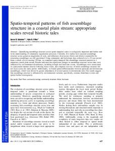
Fig. 1. Discretizing trajectories with fixed-size grids

fore temporal properties of objects are abstracted into the sequential order and redundancy of symbols [3]. Although grid-based partition is a simple and intuitive way to divide the data space, we may not obtain satisfactory results in finding spatio-temporal patterns, for several reasons. First, an inappropriate cell size results in losing important patterns. If the cell size is too large, the movements of objects inside a cell will be lost during discretization [7]. Fig. 1b shows that two different sequences are converted to the same sequence {A,A,A,A,A,A,A,A,B,D}. In this case, we may get wrong frequent patterns. On the contrary, if the space decomposition is dense, two very similar trajectories are discretized into completely different sequences, as shown in Fig. 1c. Second, small cell size and highly redundant symbols may decrease the efficiency of the mining process. The performance of the sequential mining process is closely associated with the length of sequence and the number of different items appearing in the sequences. If data space is decomposed into overly fine granularities, the number of different cells in sequences drastically increases. Moreover, as the duration of the object’s movement is represented as redundant location symbols, long sequences suffer from an inefficient mining process. Third, inaccurate and unintuitive patterns may be derived from input data. A sequence {A,…, A,B,…,B,C,…,C} has a different temporal meaning than does {A,B,C}, in that the former is intended to visit each region and spend some time; on the other hand, the latter appears to pass A, B and C as an intermediate location on its way to the destination. However, if the former is found to be a frequent pattern, the latter will also be frequent irrelevant to its actual support count due to the characteristics of the support counting step in the sequential mining process. Furthermore, long, redundant symbols may limit the interpretability of the extracted patterns. Thus, we need to represent trajectories in a better way, which efficiently deals with temporal properties. Trajectories can be partitioned into disjointed subsequences by detecting meaningful spatiotemporal changes in objects’ movement. A segment between two change points forms a spatiotemporal region, which includes both a spatial and a temporal approximation of movements within the segment. Temporal abstraction in the regions resolves the redundancy of location symbols, and enables sequences to be represented spatio-temporally, not spatio-sequentially. If original trajectories are converted as sequences of the spatio-temporal regions, a spatio-temporal pattern can be defined as follows: Definition 2. A Spatio-Temporal pattern ST = 〈R1R2...Rk〉 for k < n, such that a spatiotemporal region Ri =(si, di), si is a spatial approximation of points from tl to tm in trajectory T (l < m < n), and di is a duration of movements between tl to tm.

524


Fig. 2. Different representation of a spatio-temporal region

Fig. 2 shows two different representations of ST-patterns. As shown in Fig. 2a, spatial changes in location are approximated into a 2-dimensional rectangle, and the transition time within the segment is abstracted into the height of a 3-dimensional hyper rectangle. Therefore, we can obtain spatio-temporal regions Ri by grouping similar hyper rectangles. They incorporate spatial and temporal information into a spherical region. On the other hand, if we abstract the spatial movements of objects into a 2-dimensional cluster si, then a spatio-temporal region can be represented as a form of [si, di] (Fig. 2b), where di means the duration value between the end points. Notice that different spatio-temporal regions can be generated by adjusting the degree of spatio-temporal approximation using threshold values; segmentation threshold δ, clustering threshold εc and temporal threshold εt values. Finally, the mining ST-pattern problem searches all frequent spatio-temporal patterns in the original trajectory T, which are frequent, given a line simplification threshold δ, clustering threshold εc, temporal threshold εt and minimum support min_sup.

4. MINING SPATIO-TEMPORAL PATTERNS BY INCORPORATING TEMPORAL PROPERTIES In the previous section, we discussed that discovering ST-patterns from trajectories can be a problem of finding frequent subsequences from the sequences of spatio-temporal regions. In this section, in order to mine frequent spatio-temporal patterns from trajectories, we propose two different methods according to how the spatio-temporal region is formulated. MST-ITP (Mining Spatio-Temporal patterns by Incorporating Temporal Properties) is a straight forward approach to incorporate temporal properties into a multidimensional spherical spatio-temporal region. Another approach, MST-TEQ (MST with Temporal Quantities), treats temporal information explicitly as a form of extended pattern from the conventional sequential patterns.

4.1 Discovering Spatio-Temporal Regions In order to discover ST-patterns from trajectories, we first partition the data space into spatiotemporally meaningful regions. Also, we want to reduce the data size during discretization to improve the efficiency of the mining process. To tackle this problem, we first summarize trajecories into their approximations using line simplification. Simplified segments abstract the

525


movements of objects as well as compress the data size. Then we cluster the simplified segments into the disjointed spatio-temporal regions. Finally, original trajectories are discretized into sequences of cluster-ids into which the points of simplified trajectories fall. Line simplification is a method for abstracting poly-lines within a deterministic error boundary [12]. In our approach, we adopt a DP (Douglas-Peucker) algorithm, since it is mathematically superior to other line simplification algorithms, and also provides the best perceptual representations of the original lines. The basic DP algorithm recursively decomposes a set of points of a trajectory T:{p1, p2,…,pn} to a subset T ′ :{p'1, p'2,…,p's} ⊆ T, s ≤ n. Starting from the line segments of p1 and pn, it examines whether the farthest point from a line has a distance at most δ, a user specified threshold. If the distance is below the given threshold, then the segment formed by the two end points can be accepted as an approximation of all points between them. Otherwise, it is divided at the farthest point, and then two split parts are recursively simplified. As a result, the segment from p'i-1 to p'i approximates all the original points between them, such that the perpendicular distance from it is at most δ, as shown in Fig. 3. In order to intertwine spatial approximations from the previous phase with temporal information, we derive a feature vector v, defined as a triple, v = {Pl, Pr, d}, where Pl and Pr are the two end points of the line segments and d is a duration value for movements along the path in the corresponding segments, as shown in Fig 3. As a result, feature vectors V:{v1,…vk-1} (1 < k ≤ m1), where vk = {Pk-1, Pk, dk}are calculated from simplified trajectory T ':{p'1,…,p'm}. Since it is meaningless to compare vectors with different offsets and ranges of values, we need to equalize the importance of all features by normalization. We adopted min-max normalization which performs a linear transformation on the original data into a new range, generally [0,1]. It maps a value v to each v' by calculating v'=((v-min)/(max-min))×(newmax-newmin)+newmin). The movements of objects are not uniformly distributed in the data space. Therefore, we have to identify meaningful regions considering spatial movements of objects and their related temporal information, to partition the data space appropriately. In order to identify the regions considering the distributions of data, we cluster the simplified segments into a spatio-temporal region, as shown in Fig. 3. We can represent the spatial and temporal properties of a simplified segment as a feature vector, and adopt a clustering algorithm to find proper clusters from these vectors. It is known that the computational complexity of most clustering algorithms is at least quadratic. Furthermore, since we are interested in specifying the “closeness” threshold between clusters, we consider the pre-clustering phase of BIRCH [13] as a clustering step. The pre-clustering phase of BIRCH has linear time complexity in input size and stores a summary of data in a

Fig. 3. Feature vectors and spatio-temporal regions in MST-ITP 526


compact tree structure, or CF-tree. It incrementally scans data, and inserts points into the CFtree, building summarizations for clusters. Given the value of εc and feature vectors, our clustering phase generates groups of similar segments which divide data space into disjoint groups. The number of clusters and their size can vary based on the value of δ, εc and the complexity of original trajectories. For example, more complex trajectories tend to generate more different segments by line simplification; therefore, the number of clusters increases with the complexity of trajectories. Likewise, the size of a cluster is basically dependent upon the size of the simplified segments, but is also affected by the threshold value εc. In MST-ITP, temporal information is incorporated into a spatio-temporal region ri, which implicitly includes both spatial and temporal approximations as shown in Fig 3. Therefore, we could describe trajectories as a sequence of symbols of the spatio-temporal regions’ ids. Finally, an original trajectory T is abstracted into a sequence 〈r1r2…rk〉 of a spatio-temporal region id ri.

4.2 Mining ST-Patterns by Incorporating Temporal Properties Since we obtain the sequences of spatio-temporal regions from the original trajectories, we can discover frequent spatio-temporal patterns by applying the sequential pattern mining techniques to these sequences. MST-ITP adopts a projection-based approach from [14] for the sequences of spatio-temporal regions. It is an extension of the pattern-growth approach to mine sequential patterns from a sequence database. It first generates all length-1 patterns in the database. Then it recursively constructs projected databases and finds all frequent patterns. Our methods adopt a variant of this pattern-growth approach to mine the spatio-temporal patterns. Fig 4 illustrates the algorithm in detail. At first, it discovers a set of spatio-temporal segments

Fig. 4. MST-ITP algorithm 527


r from input trajectory database T using line simplification and clustering (line 1-3). Then, it finds frequent 1-regions (i.e., frequent 1-patterns) from the sequences of regions. All the region ids with a support count greater than the min_sup are discovered using a depth-first traversal, by extending prefixes (line 5). Starting from the discovered 1-length regions, MST-ITP discovers longer ones in a prefix-projection style. For each frequent region ri in R, we calculate the 〈r〉projected database, which consists of the set of suffixes for the prefix ri in R. By scanning the 〈r〉-projected database once, all patterns with length-2 having a prefix 〈r〉 can be generated by appending a new item to the last element (in Procedure Pattern_Extraction). Since a trajectory contains one location measurement at each time stamp, a sequence of spatio-temporal regions in R cannot have continued items (e.g. (_r1)). Therefore, it is not required to deal with continued items in constructing projection databases and in support counting. This modification enables the method to reduce unnecessary support counting steps in implementing the algorithm.

4.3 Mining ST-Patterns with Temporal Quantities As described in the previous subsection, MST-ITP does not deal with temporal information explicitly. Therefore, while the spatial granularity of an extracted pattern could be controlled by parameters, the temporal granularity could not be specified. In addition, in order to analyze precisely the results from MST-ITP, the extracted patterns need to be post-processed based on the information of spatial and temporal approximation. In this subsection, we present another version of mining algorithm MST-TEQ, which explicitly handles temporal properties and adjusts the degree of temporal approximations. In order to deal with temporal information, we formulate the duration values into the temporal quantities. In addition, to deliver the notion of temporal quantities into the pattern discovery, the mining process which discovers spatio-temporal regions should be modified. Since we are interested in describing movements of objects more precisely, we include a direction of the movement in a vector. For instance, consider two objects located in the same area moving towards the opposite direction at any timestamp t. Although they are at the same location, their meanings of movement are apparently different. A value of relative angle between segments can be a good descriptive explanation of difference for line segments. Therefore, feature vectors v are defined as a triple, v = {Pl, Pr, θ}, where Pl and Pr are the two end points of the line segments and θ is the degree of angle formed by a line segment from Pl to Pr and the x-axis, as shown in Fig 5. MST-TEQ also adopts the pre-clustering phase of BIRCH to cluster spatial segments into groups. As shown in Fig. 5, groups of spatial regions form a circular cluster in R2 and temporal properties of the cluster are depicted by the height of the cylinders. Therefore, we could describe spatio-temporal regions as a pair of [sid, d]. We finally obtain sequences of the pairs after the clustering step, which abstracts movements of the objects in original trajectory T. Since we first decompose the original trajectories into spatial approximations, a series of regions with the same spatial symbol but different temporal quantities, may be generated. In order to optimize the mining performance by reducing the length of sequences, we merge two consecutive spatial regions with the same symbol si into one, adding two duration values. For example, a sequence 〈[s1,0.1] [s1,0.1]…[s3,0.05]〉 could be simplified into 〈[s1,0.2]…[s3,0.05]〉 by merging duration values of s1. Continuous values of temporal properties have to be discretized to be applied to sequential pattern mining algorithms. The simplest way to discretize continuous values is to construct a histogram based on error minimization. However, it is still possible for similar values to be as-

528


Fig. 5. Feature vectors and spatio-temporal regions in MST-TEQ

signed to different buckets. We adopt the BIRCH pre-clustering phase to discretize temporal properties. Our method finds a proper partition of the temporal domain by clustering similar values into a group based on the temporal threshold εt. Finally we have a sequence of spatiotemporal regions ST = 〈[s1,d1][s2,d2]…[sk,dk]〉, where si is a symbolic id of spatial approximation and di is the discretized temporal quantity of continuous duration value, for 0 ≤ di < 1. Then, the problem is considered as extracting frequent quantitative sequential patterns given a sequence database. So far, although not much work has been done in the quantitative sequential pattern mining domain, [15] studied the discovery of frequent patterns from market basket data with quantity constraints. However, temporal quantity should be treated differently than the conventional quantity constraints, since duration values mean different things. Therefore, a performance optimization by pruning infrequent temporal quantities based on inclusion relationships is not possible. Although 0.01 < 0.5 is a quantitative relationship, [s1,0.01] should not be filtered even when [s1,0.5] is not a frequent item. Based on this observation, we have to extend a prefix projection-based algorithm in several respects. (a) Constructing a projection database: Since a spatio-temporal sequence consists of discrete symbols of spatial temporal quantities, the notion of an item in a conventional PrefixSpan algorithm should be extended into a form of [si, di]. To support this kind of extension, we generate projected databases for all possible combinations of frequent si and di. (b) Continued items: A trajectory contains one location measurement at each time stamp, the discretized sequence of the original trajectory cannot have continued items (e.g. (_s1)). Therefore, it is not required to deal with continued items in constructing projection data bases and in support counting. Fig. 6 describes the MST-TEQ algorithm and the Ext_Pattern_Extraction procedure in detail. At first, we partition the data space by finding spatio-temporal regions using line simplification and clustering as described in the previous subsection. Then, we merge the duration values of the same spatial property and discretize them into the discrete temporal values (line 4-5). Starting from all extended items of [sid, d] with a support count greater than the min_sup, the Ext_Pattern_Extraction procedure is recursively executed to generate projection databases. Then we generate extended frequent patterns F'α with all possible temporal quantities. For all the

529


Fig. 6. MST-TEQ Algorithm

patterns s in S, the procedure is recursively executed with new prefixes. Finally, MST-TEQ finds frequent patterns based on the extended patterns based on all possible temporal quantity values.

5. EXPERIMENTS In this section, we provide an experimental evaluation of the proposed methods. Due to the lack of real data from privacy issues, we use synthetic datasets for the test. The language used was C++ in implementing the algorithm and experiments were performed on a Pentium D 3.4 GHz machine with 1GB memory. We used the C++ library of geometry functions for implementing line simplification and several distance functions. The pre-clustering phase of BIRCH is implemented based on the original paper [13] and source code provided on the site: http://pages.cs.wisc.edu/~vganti/birchcode/

530


5.1 Datasets and Experimental Settings In order to evaluate the performance of methods under different data distributions, we generated synthetic data using spatio-temporal data generator G-TERD [15]. It is a highly parameterized and flexible generator for simulating the objects’ movements with realistic scenarios. The important parameters are the number of time slots (TS), which is the length of the time history in a trajectory, the number of scenarios (NS) describing movement patterns of objects, the number of objects per scenario (NO), and the distribution (D) of the center. The characteristics of datasets and parameter settings were summarized in Table 1. Other parameters are set to the default values suggested in [15]. Generated data is distributed in a workspace of 1000×1000 units. We used two different existing methods, GSP and PrefixSpan, in the comparison of the mining results. For both cases, we discretized input data into a sequence of location symbols using equal width discretization (EQW), which are mostly used in existing spatio-temporal mining studies. The GSP [17] and PrefixSpan [12] discover sequential patterns from a transactional database by a breadth-first and depth-first search, respectively. The PrefixSpan binary code and the GSP1 open source code were used for the tests. Table 1. Datasets and the settings Datasets

Size

SN

TS

NO

Description

SN1_TS40_NO40

1.6K

1

40

40

Mining quality test

SN5_TS1000_NO#

1K~5K

5

1000

20-100

Scalability test

SN4_TS100_NO25

10K

4

100

25

Impact of simplification test

5.2 Mining Quality In order to test the capability of our approach in discovering accurate frequent patterns from input data, we compared the extracted patterns with GSP and PrefixSpan. Fig. 7a and 7b show input trajectories in a 2- and 3-dimensional view, respectively. The dataset consisted of partial gularities and noises. We set min_sup to 0.2, δ to 0.025, εc to 0.0035, and εt to 0.1, respectively. As all values are normalized into vectors between 0 and 1, threshold values are also set to the values between them. As we mentioned earlier, data space is divided by n×n cells, we vary n to 5 (grid5) and 20 (gird20). Fig. 8 shows max-patterns extracted by GSP and PrefixSpan, when the data space is partitioned into grid5 and grid20 respectively. Note that, although GSP and PrefixSpan have different execution times, they generate the same max-pattern. We plot the direction of the movement among cells as arrows. The max-pattern from the proposed methods is illustrated in 2 and 3dimensional views in Fig. 9. The movement patterns of the original trajectories are successfully derived by our methods and by GSP with grid20, as shown in Fig. 8b and 9a. However, with the coarse grid (grid5), the movement of small displacement in the cell of the left bottom corner is lost (Fig. 8a), while our method clearly captures the movements with segments s1s7 in Fig 9a. Although we can derive accurate patterns using a dense grid, the search space drastically increases due to the processing of a large number of different items (cell ids) in sequences. We now compare the compactness of extracted patterns. As we can see in Fig. 9, MST-TEQ discovers regularities in data, as a compact pattern 〈s1s1s7s11s9s10〉. As we expected, segments 1 available at http://illimine.cs.uiuc.edu/download/ and http://cs.uwindsor.ca/~cezeife/plwapcode.tar.gz

531


(a)

(b)

Fig. 7. Input trajectories in 2-dimensional and 3-dimensional view

(a)

(b)

Fig. 8. The maximal patterns extracted from GSP and PrefixSpan

(a)

(b)

Fig. 9. The maximal patterns extracted from proposed methods (MST-TEQ)

with similar movements are grouped into a region and decomposition occurs at spatiotemporally meaningful points. On the other hand, much longer and unintuitive patterns with

532


Table 2. Extracted maximal patterns and the execution time Methods

Maximal patterns

Length

Execution time

MTP-ITP

{r8,r2,r3,r4,r6}

5

0.02

MTP-TEQ

{(s1,7)(s1,7)(s7,6)(s11,5)(s9,8)(s10,7)}

6

0.15

34

33.6

28

98.3

Prefix 5×5 grid {C2C2C2C7…C7(18)C8C13C13C14C14C19C19C18C18C22C22C22C22C17} Span/ GSP 20×20 {C66C66C86C85C85C85C85C105C106C106C106C106C106C106C106C107C128C171C192 grid C213C254C273C310C328C347C326C285}

redundant symbols, of length-34(grid5) 〈c2 c2…c22 c17〉 and of length-28 (grid20) 〈c66 c66…c326 c285〉 are extracted by GSP and PrefixSpan. Similarly MST-TEQ extracts a 5-length pattern 〈r8r2r 3r 4r6〉 as a result. Almost all regions have similar temporal duration values, which include 6 to 11 points as shown in Fig. 9b, MST-TEQ generates only two temporal clusters [0−0.2] and [0.2−0.25] with the given temporal threshold εt = 0.1. We observed that when we set the temporal threshold under the certain threshold, in this case 0.06, the maximal pattern cannot be detected and shorter sub-patterns of the maximal are obtained. As MST-IPT and MST-TEQ transform the original trajectories into compact representations before the pattern mining process, they perform better than the existing approaches as shown in Table 2. Actually, in MST-TEQ, values of temporal duration are normalized to values between [0,1], but to analyze the results more precisely, we provide the values before the normalization, that is, the number of points. The execution times of GSP and PrefixSpan grow much faster than the proposed algorithms, especially when the trajectories are long and complex. As shown in Table 2., as MST-IPT extracts accurate patterns considering spatio-temporal changes in the original data, post-processing for calculating temporal durations of each spatio-temporal region is needed in order derive the exact temporal information from the extracted pattern. On the other hand, MST-TEQ provides the travel times of region explicitly, thus patterns from MST-TEQ give us more intuitive and easily understandable results.

5.3 Mining Efficiency In the next set of experiments, we study the scalability of the proposed methods with respect to data size, by comparing total execution time. We use datasets SN1_TS1000_NO20~100 as input and run scale up experiments under two different min_sup values. We set δ to 0.06, εc to 0.04, and εt to 0.05 and use grid10 for EQW discretization in order to obtain the running time in a comparable scale. With grid20, the performance difference between our methods and the others becomes too large, and it is difficult to compare the results together. Fig. 10 plots the execution time of all methods. As we expected, our approaches show a significant increase in speed over the other methods as the data size increases. Since the performance of the mining process is highly associated with the length of the sequences and the number of different symbols in sequences, the abstracted representation of our methods reduce the data size and prune the search space in the mining process. Observe that as the min_sup value decreases, the performance gap between our methods and the others becomes more significant (Fig. 10b).

533


(a) min_sup = 0.5

(b) min_sup = 0.3

(c) Execution time with min_sup

Fig. 10. Mining efficiency under different data size and min_sup

5.4 The Impact of Approximations The last experiment examines the impact of spatial and temporal approximations of the proposed methods with respect to the increased threshold values δ, εc, and εt. The number of simplified segments and the size of cluster are determined by corresponding threshold values, that is δ and εc. In existing approaches, the size of grid affects considerably the results of discretization and mining. Similarly, the size of simplified segments and generated clusters is closely related to the accuracy of the mining results. Fig. 11 plots the execution time for increasing threshold values. For testing the impact of δ, we set min_sup to 0.2 and εc to 0.04. No change in min_sup and δ to 0.001 for testing εc. The settings for testing the impact of εt is that δ = 0.01, εc = 0.04 and min_sup = 0.15. As we increase the threshold δ, the boundary of the spatial area becomes large, thus a smaller number of simplified segments are generated for each trajectory. Consequently, the length of sequence of spatiotemporal regions decreases as the δ grows. Therefore, as the δ increases, we expect that the running time of the mining process will decrease, which is compatible with Fig. 11a. Similarly, as the εc increases, more segments are grouped into one cluster and the number of different regions is reduced. Although they do not have a linear relationship, Fig. 11b illustrates that the execution time phases down as the εc increases. Finally, we observe the impact of temporal threshold values on mining performance. As the temporal threshold value εt increases, the number of temporal segments decreases and finally becomes one, when the value is over a certain threshold. That is, when all the temporal values are assigned into the same bucket. The dras-

(a) Simplification threshold

(b) Clustering threshold

Fig. 11. The impact of approximation on mining performance

534

(c) Temporal Threshold


tic increase in the execution time around the εt value 0.06 in Fig. 11c, results from the fact that all the temporal approximations of spatio-temporal regions have the same value, and thus the possibility of finding patterns with the given min_sup is escalated. We argue that there is a tradeoff between mining performance and the descriptive power of extracted patterns, since patterns may be lost if the approximation is overly coarse. Therefore, we have to adjust the range of threshold values considering the original distribution of input data.

6. CONCLUSION In this paper, we presented an approach for mining spatio-temporal patterns from trajectory data. We introduced the problem of representing spatio-temporal properties with redundant location symbols. Sequential descriptions of temporal properties degrade the mining efficiency and the compactness of extracted patterns. To address this problem, we proposed an efficient method for mining spatio-temporal frequent patterns. First, we defined a spatio-temporal pattern by approximating spatial and temporal properties. Regarding how to integrate spatial and temporal properties, spatio-temporal patterns are represented as a sequence of multidimensional regions of a sequence of pairs of [spatial approximation, duration]. Based on these definitions, we proposed two different methods − MST-ITP and MST-TEQ − to discover frequent spatio-temporal patterns. The proposed methods first abstract original trajectories into simplified segments using line simplification then generate sequences of spatio-temporal regions using clustering from the simplified segments. Finally, spatio-temporal frequent patterns are extracted in a prefixprojection approach. By abstracting spatio-temporal information into efficient representations, the search space for the mining process considerably decreases. In addition, by reducing the length of sequences and the number of different symbols appearing in sequences, our methods extract more intuitive patterns. Experimental results demonstrate the efficiency and effectiveness of our methods when compared to the existing approaches. Future work is needed for selecting the threshold values more intelligently based on the distribution of input data and for experiments with practical real data sets.

REFERENCES [1] [2]

[3] [4] [5] [6] [7]

G. Gidófalvi, T. Pedersen, “Mining Long, Sharable Patterns in Trajectories of Moving Objects”, Proceedings of STDBM, 2006, pp.49-58. J. Kang, and H. Yong, “Spatio-temporal discretization for sequential pattern mining”, Proceedings of International Conference Ubiquitous Information Management and Communication, 2008, pp.218224. I. Tsoukatos, and D. Gunopulos, “Efficient mining of spatiotemporal patterns”, Proceedings of International Symposium on in Spatial and Temporal Databases, 2001, pp.425-442. D. Birant and A. Kut. “ST-DBSCAN: An algorithm for clustering spatial-temporal data”, Data and Knowledge Engineering, Vol.60, No.1, 2007, pp.208-221. V. S. Tseng, K.W. Lin, “Mining Temporal Moving Patterns in Object Tracking Sensor Networks”, Proceedings of International Workshop on Ubiquitous Data Management, 2005, pp.105-112. G. Yavas, D. Katsaros, O. Ulusoy, and Y. Manolopoulos. “A data mining approach for location prediction in mobile environments”, Data and Knowledge Engineering. Vol.54, No.2, 2005, pp.121-146. N. Mamoulis, H. Cao, G. Kollios, M. Hadjieleftheriou, Y. Tao, and D. W. Cheung, “Mining, indexing, and querying historical spatiotemporal data”, Proceedings of 10th International Conference on

535


[8] [9] [10] [11]

[12]

[13] [14]

[15] [16] [17]

Knowledge Discovery and Data Mining, 2004, pp.236-245. H. Cao, N. Mamoulis, and D.W. Cheung, “Mining frequent spatio-temporal sequential patterns”, Proceedings of Data Mining, 2005, pp.82-89. H. Cao, N. Mamoulis, D.W. Cheung, “Discovery of Periodic Patterns in Spatiotemporal Sequences”, IEEE. Transactions on Knowledge and Data Engineering, Vol.19, No.4, 2007, pp.453-467. F. Giannotti, M. Nanni, D. Pedreschi, and F. Pinelli, “Trajectory Pattern Mining”, Proceedings International Conference on Knowledge Discovery and Data Mining, 2007, pp.330-339. A. Monreale, F. Pinelli, R. Trasarti and F. Giannotti, “WhereNext: a Location Predictor on Trajectory Pattern Mining,” Proceedings of the 15th ACM SIGKDD International Conference on Knowledge Discovery and Data Mining, 2009, pp.637-646. J. Pei, J. Han, B. Mortazavi-Asl, H. Pinto, Q. Chen, U. Dayal, and M.C. Hsu. “PrefixSpan: Mining sequential patterns efficiently by prefix-projected pattern growth”, Proceedings of 17th International Conference on Data Engineering, 2001, pp.215-224. H. Cao, O. Wolfson, and G. Trajcevski, “Spatio-temporal data reduction with deterministic error bounds”, The VLDB Journal, Vol.15, No.3, 2006, pp.221-228. T. Zhang, R. Ramakrishnan, and M. Livny, “BIRCH: An efficient data clustering method for very large databases”, Proceedings of ACM SIGMOD International Conference on Management of Data, 1996, pp.103-114. C. Kim, J. Lim, R. T. Ng, and K. Shim, “SQUIRE: Sequential Pattern Mining with Quantities”, Journal of Systems and Software, Vol.80, No.10, 2007, pp.1726-1745. T. Tzouramanis, M. Vassilakopoulos, and Y. Manolopoulos. “On the generation of time-evolving regional data”, Geoinformatica, Vol.6, No.3, 2002, pp.207-231. R. Srikant and R. Agrawal. “Mining Sequential Patterns: Generalizations and Performance Improvements”, Proceedings of the 5th International Conference on Extending Database Technology, 1996, pp.3-17.

Juyoung Kang She received her B.E., M.E., Ph.D degrees in Computer Science and Engineering from Ewha Womans Univ. in 1999, 2001 and 2010, respectively. During 2003 to 2005, she served as a as a research member at Korean Electric Power Research Institute and a senior researcher at Neomtel co. for industrial experience. Her research interests include data mining, especially spatio-temporal data mining, and information retrieval.

Hwan-Seung Yong Hwan-Seung Yong is a Professor of Computer Science and Engineering at Ewha Womans University, Republic of Korea since 1995. He received his B.S., M.S. and Ph.D. degrees in Computer Engineering from Seoul National University. He has five years of industrial experience as a Researcher at ETRI (Electronics and Telecommunications Research Institute) and served as a visiting scientist at the IBM T.J. Watson Research Center. He is a member of KIISE (The Korean Institute of Information Scientists and Engineers) and ACM. His current major research interests include agile methods, data mining, multimedia databases and ontology searches.

536