Uluslararası Mühendislik Araştırma ve Geliştirme Dergisi International Journal of Engineering Research and Development Cilt/Volume:10
Sayı/Issue:2
Haziran/June 2018
https://doi.org/10.29137/umagd.376895
Araştırma Makalesi / Research Article
.
Mixed Noise Removal with External Parameter in Image Denoising Uğur ERKAN1, Levent GÖKREM*2 1Erbaa Vocational School, Gaziosmanpasa University, 60500 Erbaa, Tokat, Turkey . 2The Faculty of Engineering and Natural Sciences, Gaziosmanpasa University, 60100 UPM, Tokat, Turkey
Başvuru/Received: 10/01/2018
Kabul/Accepted: 13/06/2018
Son Versiyon/Final Version: 29/06/2018
Abstract In this study, a new method has been developed on noise removal, one of the most important parts in image processing. In particular, a new noise removal filter has been developed to removes noise from images the mix of µ and σ values. In this method, a new approach is proposed to remove noise when μ value increases while σ value is constant. The filter has particularly proven to be more successful on all of µ values. PSNR have been used to compare the results of the study. The newly developed method has been compared with the median, wiener2, Bayesian shrink, bilateral, median+bilateral, BM3D, KSVD methods. For example, when µ-0.10 and σ-0.01 added to Lena image, other algorithms’ PSNR results are 19.23-19.35, 18.90, 18.73, 19.60, 19.81, 19.70 while they are 27.06 in our new method.
Key Words Gaussian Noise, Image Denoising, Noise Removal, Image Enhancement
[email protected]
International Journal of Research and Development, Vol.10, No.2, June 2018
1.
INTRODUCTION
While digital imaging technology plays a major role in areas such as satellite televisions, resonance imaging, and computed tomography as well as in application areas such as geographic information systems and astronomy. Image denoising is vital in image processing and machine vision, and in time it continues to gain importance Rafsanjani vd., (2017). Generally, the data accumulating in the image sensors is contaminated by noise during the image acquisition and digital transmission stage Sakthidasan vd., (2016), Chen vd., (2014), Garnett vd., (2005). In other words, noise occurs in these images during digital image acquisition and transfer processes (Zhang & Wang, 2015). Images are contaminated mostly with Gaussian noise during digital image acquisition processes. One of the most important stages of image enhancement is to remove the noise from the image. However, what is more important in image processing is to be able to conserve the features of the original image while removing the noise Garnett vd., (2005), Montagner vd., (2014), Liu vd., (2008), Khana vd., (2016). One of the most well-known noise removal methods is algorithms based on Partial Differential Equations, neighbourhood filters and the noise detection Bouboulis vd., (2010), Khmag vd., (2016). Different filters are also developed according to the type of noise. The filters based on predicting the noise density are quite popular, yet they have still a major setback; these filters cannot remove noise from images in real-time applications (Liu & Lin, 2013). Gaussian and impulse noise are two of the most studied noise-types. As for impulse noise, pixels contaminated with noise are converted to a maximum or a minimum value of signal (Lopez-Rubio, 2010), (Erkan & Kilicman, 2016). As for Gaussian noise, each pixel is increased or decreased in a certain amount, and Gaussian Distribution Model having a zero mean feature simulates this type of noise very well Jaiswal vd., (2014). Gaussian noise is added to images using imnoise function in matlab software. With imnoise function, data randomly generated with Gaussian distribution is added to the image Xiao vd., (2011). One of the most popular and effective methods for removing noise from images is standard median filter (SMF). In this filter, pixels are sorted in ascending order, and then the median pixel value becomes the new pixel value. This filter does not preserve original pixel values; however, it gives good results, but SMF creates a blurred effect on image Xiao vd., (2011), Huang vd., (2009). One of the effective ways to remove the Gaussian noise is the wiener filter, a function of matlab. Wiener filter is a linear filter that reduces the amount of noise and image blur, and minimizes the mean square error. However, a disadvantage of the method is that it requires prior information about the original image, which does not exist in any real-time application. It also does not allow exchanges between dense and flat areas. Therefore it is not suitable for images with a high volume of blurred area Vijaykumar vd., (2010). Bilateral filtering determines the new pixel value, based on any given pixel space and range value, which helps conserve edge and pixel properties. Bilateral filtering is local, nonlinear, non-iterative method that uses the information of gray level photometric similarity and neighbouring pixels’ geometric closeness (Tomasi & Manduchi, 1998), (Kumar, 2013). Main objective with bilateral filter is to extract edge properties and obtain a smoother area. The bilateral filter that is a nonlinear filter removes the Gaussian noise, retaining the sharpness of the edges. New pixel value is found by replacing weight averages of neighbouring pixels. Weight function, while retaining the edge properties, creates new pixel value based on smoothness in the regions of similar density of central pixel and neighbouring pixels Garnett vd., (2005). Sparse 3D transform-domain collaborative filtering (BM3D) to remove the Gaussian noise is a method generating good results. BM3D is a three-stage process as follows; block-matching and grouping, collaborative filtering, aggregation and estimation. First, grouping is performed by block-matching, and the collaborative filtering is accomplished by shrinkage in a 3D transform domain. Finally, in aggregation and estimation, new pixel value is found with a locally obtained prediction based on weight average, considering all the data so far obtained Montagner vd., (2014), Dabov vd., (2007), (Chong & Zhu, 2013), Chang vd., (2000). Bayesian Shrink is a method that eliminates square error by minimizing Bayesian risk thus removing image noise Chang vd., (2000). This method is rather successful in removing noise from medical and natural images Khmag vd., (2016). KSVD is the generalized form of K-means clustering process. KSVD, an iterative method, updates the image data with dictionary atoms to better fit and then updates the dictionary itself. To remove the noise, this method uses representation in terms of the dictionary in image denoising Aharon vd., (2006), Golestani vd., (2014). KSVD through learning the dictionary removes additive white Gaussian noise image from gray scale images. Sparse representation models offer another powerful method to analyse images based on the sparsity and redundancy of their representations. This type of models, using training dictionary for each small block, makes assumptions related with existing sparse linear combination. This linear combination is created through KSVD algorithm’s extracting training algorithm from noise images Liu vd., (2013). In this paper, we have developed a new method to remove the Gaussian noise from images. In removing the noise, this new method has been applied to images to which both μ and σ values are added with imnoise function. In this new method, windowing and neighbourhood noise removal methods are used. New pixel value is decided by looking at standard deviation and the mean of 136
International Journal of Research and Development, Vol.10, No.2, June 2018
pixels that are grouped horizontally and vertically after windowing. Different noise density with an input parameter (k) is intended to produce new values. 2.
PROPOSED ALGORITHM
To remove noises, a new method has been developed in which the µ value increases while the σ value is constant at the Gaussian noise. Constant number (k), an external parameter, is used to estimate noise density while μ value is increase. To remove the noise, square windowing is done. Firstly, two new matrices are created from the pixels entering the window. The first matrix is formed by the horizontal and vertical neighbors of the center pixel. The second matrix is the window itself. The mean and standard deviation values of the two newly created matrices are be calculated. Then, if the noisy pixel value in the center of the window is within or outside the range provided in the 4th step, two new equations are used to find the new pixel value (shown in Step 4 below). New pixel value is calculated the using the mean and standard deviation values of 2 matrices. Fig. 1 shows the flowchart of the new method. Two matrixes are formed according to the window size given as a parameter (for example; window size 3x3). A new matrix is formed with pixels used for matrix 1 and matrix 2 in Fig. 2.
Figure 1. New Method Flowchart
Nestled in flowchart;
Ve , processing incoming pixels Vnew _ value , new pixel value after processing
µ1 , µ2 , σ 1 , σ 2
will be described in the algorithm steps.
137
International Journal of Research and Development, Vol.10, No.2, June 2018
At later stages, the implementation steps of the algorithm steps are explained. The window size was 3x3 and the equations were created accordingly. Step 1. Form Matrix 1 and Matrix 2 from 3x3 windowing
Figure 2. Matrix 1 and Matrix 2 formation
Step 2. If we use µ1 and µ2 for average, µ1 for Matrix 1, µ2 for Matrix 2
µ1=
1 3 ∑a2i + bi 2 m i =1
(1)
1 2 ∑aij mn i , j =1
(2)
µ2 =
m and n are the window sizes. Step 3. For standard deviation,
σ1
= σ2
2 2 ∑ ( a2i − µ1 ) + ( bi 2 − µ1 ) , 1 ≤ i ≤ 3 ( ) m
∑ ( aij − µ2 ) m
(3)
2
, (1 ≤ i, j ≤ 3)
(4)
Step 4. If we show the pixel value processed with
Ve and the new pixel value with Vy ,
138
International Journal of Research and Development, Vol.10, No.2, June 2018
if V & Ve < µ1 + k e > µ1 − k
(5)
Vy = µ1 + σ 1 + σ 2 − k
(6)
If not, it becomes
Vy = µ1 − σ 1 − σ 2
(7)
k here is the external parameter determined by the noise density. Parameter k is a constant number. k values were found according to noise intensities. Parameter k value increases as noise increases. Parameter k is constant number when image noise density reaches a certain value. For all values with µ greater than or equal to 50 % are 73 of k k value.
3.
ALGORITM RESULTS
3.1.
Algorithm Evaluation Criteria
In this study, 18 images were used to test the newly proposed method. These images are used commonly to test denoising methods. 1 criterion is used to assess the results of the algorithm. The Mean Squared Error (MSE) is needed in calculation of the PSNR (Peak Signal- to-Noise Ratio) value. MSE;
= MSE
2 1 m −1 n −1 I ( i, j ) − K ( i, j ) ∑∑ mn=i 0=j 0
(8)
I is mxn image without noise. K is noise added image.
MAX I2 PSNR = 10 log10 log( ) MSE Here,
(9)
MAX I is the maximum value that a pixel in the image can get. If 8 bit is used for pixels, this value is 255 Luisier vd.,
(2010). Table 1 and Table 2 show PSNR results of eighteen test images. Table 1 is applied to
µ − 0.10, σ = 0.01 values. Table 2
0.50 and σ 0.01 . The newly developed filter in high-density Gaussian noise, as shown = shows results for= values for µ in Table 1 and Table 2, produces more successful results than other methods. PA stands for the new algorithm, Proposed Algorithm. Table 1. Test Images PSNR Results µ-0.10, σ=0.01, k=26
SMF
Wiener2
Bayesianshrink
Lena
19,23
19,35
18,90
18,73
19,60
Cameraman
19,27
19,32
18,83
18,73
Barbara
18,37
19,04
18,51
Peppers
19,20
19,32
Plane
19,26
19,95
Baboon
18,98
Bridge
KSVD
PA
19,81
19,70
27,06
19,64
19,71
19,52
26,53
18,52
18,60
19,61
19,41
23,01
18,86
18,75
19,63
19,68
19,51
27,08
19,45
19,19
19,57
20,16
20,20
26,63
19,13
18,54
18,36
18,87
19,24
19,19
23,83
18,75
19,11
18,62
18,51
18,78
19,24
19,15
23,10
Pirate
19,09
19,21
18,71
18,60
19,38
19,48
19,29
25,86
Elaine
19,25
19,42
19,01
18,88
19,68
19,78
19,63
27,06
Boat
19,06
19,25
18,75
18,62
19,30
19,54
19,37
25,11
Lake
19,13
19,44
18,91
18,75
19,38
19,64
19,56
24,96
139
Bilateral SMF+Bilateral BM3D
International Journal of Research and Development, Vol.10, No.2, June 2018
Table 1(cont). Test Images PSNR Results Flintstones
19,17
19,65
19,08
18,96
19,06
20,03
19,88
20,12
Living Room
19,00
19,20
18,69
18,56
19,19
19,52
19,33
25,01
WomanBlonde
19,06
19,25
18,74
18,67
19,39
19,58
19,38
25,82
WomanDark Hair
19,52
19,63
19,26
19,08
20,00
20,05
19,87
27,93
House
19,44
19,70
19,31
19,06
19,88
20,09
20,00
28,78
Parrot
19,27
19,44
18,97
18,89
19,67
19,86
19,65
26,18
Flower
19,15
19,24
18,71
18,57
19,41
19,56
19,35
25,63
µ-0.50, σ=0.01, k=73
SMF
Wiener2
Bayesianshrink
Bilateral
SMF+Bilateral
BM3D
KSVD
PA
Lena
7,15
7,33
7,27
7,25
7,15
7,32
7,33
17,18
Cameraman
7,38
7,53
7,47
7,46
7,37
7,53
7,53
17,69
Barbara
7,03
7,24
7,21
7,16
7,01
7,26
7,25
16,38
Peppers
7,14
7,27
7,21
7,20
7,14
7,27
7,27
17,22
Plane
10,29
10,46
10,42
10,37
10,26
10,45
10,43
12,50
Baboon
7,04
7,32
7,28
7,19
7,00
7,27
7,27
17,84
Bridge
6,90
7,08
7,05
6,99
6,88
7,05
7,03
15,60
Pirate
6,82
6,99
6,95
6,91
6,81
6,92
6,92
17,97
Elaine
7,47
7,67
7,62
7,60
7,47
7,66
7,67
16,46
Boat
7,29
7,52
7,48
7,43
7,27
7,47
7,48
18,19
Lake
7,73
7,83
7,75
7,75
7,72
7,82
7,82
14,48
Flintstones
7,92
8,13
8,07
8,00
7,85
8,12
8,11
12,16
Living Room
6,88
7,12
7,09
7,02
6,86
7,11
7,10
18,13
Woman Blonde
7,49
7,68
7,63
7,60
7,48
7,67
7,68
17,64
Woman Dark Hair
7,08
7,16
7,10
7,11
7,09
7,17
7,17
15,64
House
7,75
7,89
7,82
7,81
7,75
7,89
7,89
14,63
Parrot
6,92
7,08
7,03
7,00
6,93
7,08
7,07
15,63
Flower
6,47
6,67
6,64
6,58
6,46
6,66
6,67
18,54
Table 2. Test Images PSNR Results
Fig. 3 shows the images of the improved filter after the removal of the noise, following the application of µ − 0.10 and σ − 0.01 Gaussian Noise to the Lena image. Fig. 4 shows the images of the improved filter after the removal of the noise, following the application of µ-0.10 and σ-0.01 Gaussian Noise to the peppers image.
Figure 3. Lena images with noise, and Lena images after noise removal
140
International Journal of Research and Development, Vol.10, No.2, June 2018
Figure 4. Peppers Image Filter Results a) Original Image b) µ-0.30, σ=0.01 noise added image c) SMF d) Wiener2 e) Bayesianshrink f) Bilateral g)SMF+Bilateral h) BM3D i) KSVD j) PA
Fig. 5 shows the success to remove Gaussian noise from Lena, cameraman, peppers and plane images where density µ from 0.10 to 0.90 and σ=0.01. The results with the highest and smallest values from tested algorithms are shown in the graphics. Fig. 5 (a) (b) - (c) shows PSNR results of our newly developed method and that among other methods, bilateral generates the lowest results and BM3D generates the highest results. Fig. 5 (d) shows PSNR results of our newly developed method and that the lowest and the highest outcomes among other methods belong to bilateral and KSVD.
Figure 5. a) Lena PSNR graph b) Cameraman PSNR graph c) Peppers PSNR graph d) Plane PSNR graph
141
International Journal of Research and Development, Vol.10, No.2, June 2018
4.
CONCLUSION
The PA method is more successful than other methods as seen in PSNR results. Our PA makes sure that the filter does not always produce the same result each time by sending an external parameter to the filter. Thus, an alternative has been designed to measure and evaluate the success of the system in real-time applications. It has been found that in real-time applications where noise is generated at the same rate, better results have been obtained for noise removal and enhancement by changing k values. The improved filter IS USED in removing high density µ and σ values, which is the most difficult task in image denoising. The success of the filter can be increased providing the suitable parameter. REFERENCES Aharon M., Elad M. and Bruckstein A., (2006). “K-SVD: An Algorithm for Designing Overcomplete Dictionaries for Sparse Representation”, IEEE Transactions On Signal Processing, 54(11): 4321-4332. Bouboulis P., Slavakis K. and Theodoridis S., (2010). “Adaptive Kernel-Based Image Denoising Employing Semi-Parametric Regularization”, IEEE Transactions on Image Processing, 19(6): 1465-1479. Chang S. G., Yu B. and Vetterli M., (2000). “Adaptive Wavelet Thresholding for Image Denoising and Compression”, IEEE Transactions On Image Processing, 9(9): 1532-1546. Chen B., Liu Q., Sun X., Li X. and Shu H., (2014). “Removing gaussian noise for colour images by quaternion representation and optimisation of weights in non-local means filter”, IET Image Processing, 8: 591-600. Chong B. and Zhu Y.K., (2013). “Speckle reduction in optical coherence tomography images of human finger skin by wavelet modified BM3D filter”, Optics Communications, 291: 461-469. Dabov K., Foi A., Katkovnik V. and Egiazarian K., (2007). “Image denoising by sparse 3D transform-domain collaborative filtering”, IEEE Transactions on Image processing, 16(8): 2080-2095. Erkan U. and Kilicman A., (2016). “Two new methods for removing salt-and-pepper noise from digital images”, ScienceAsia 42: 28-32. Garnett R., Huegerich T., Chui C. and He W., (2005). “A universal noise removal algorithm with an impulse detector”, IEEE Transactions on Image Processing, 14(11): 1747-1754. Golestani H. B., Joneidi M. and Sadeghii M., (2014). “A Study on Clustering for Clustering Based Image De-Noising”, Journal of Information Systems and Telecommunication, 2(4): 196-204. Huang Y. M., Michael. K. Ng. and Wen Y.W., (2009). “Fast Image Restoration Methods for Impulse and Gaussian Noises Removal”, IEEE Signal Processing Letters, 16(6): 457-460. Jaiswal A., Upadhyay J. and Somkuwar A., (2014). “Image denoising and quality measurements by using filtering and wavelet based techniques”, (AEU) International Journal of Electronics and Communications 68: 699-705. Khana A., Waqas M., Ali M. R., Altalhi A., Alshomrani S. and Shimd S., (2016). “Image denoising using noise ratio estimation, K-means clustering and non-local means-based estimator”, Computers and Electrical Engineering, 54: 370–381. Khmag A., Ramli A. R., Hashim S. J. and Al-Haddad S. A. R., (2016). “Additive Noise Reduction in Natural Images Using Second-Generation Wavelet Transform Hidden Markov Models”, IEEJ Transactions on Electrical and Electronic Engineering, 11: 339-347. Kumar B. K. S., (2013). “Image denoising based on gaussian/bilateral filter and its method noise thresholding”, Signal, Image and Video Processing, 7(6): 1159-1172. Liu C., Szeliski R., Kang S. B., Zitnick C. L. and Freeman W. T., (2008). “Automatic Estimation and Removal of Noise from a Single Image”, IEEE Transactions on Pattern Analysis and Machine Intelligence, 30(2): 299-314. Liu J., Tai X. C., Huang H. and Huan Z., (2013). “A Weighted Dictionary Learning Model for Denoising Images Corrupted by Mixed Noise”, IEEE Transactions on Image Processing, 22(3): 1108-1120. Liu W. and Lin W., (2013). “Additive White Gaussian Noise Level Estimation in SVD Domain for Images”, IEEE Transactions on Image Processing, 22(3): 872-883. 142
International Journal of Research and Development, Vol.10, No.2, June 2018
Lopez-Rubio E., (2010). “Restoration of images corrupted by Gaussian and uniform impulsive noise”, Pattern Recognition, 43: 1835–1846. Luisier F., Vonesch C., Blu T. and Unser M., (2010). “Fast interscale wavelet denoising of Poisson-corrupted images”, Signal Processing 90: 415–427. Montagner Y. L., Angelini E. D. and Marin J. C. O., (2014). “An unbiased risk estimator for image denoising in the presence of mixed poisson–gaussian noise”, IEEE Transactions on Image Processing, 23(3): 1255-1268. Rafsanjani H. K., Sedaaghi M. H. and Saryazdi S., (2017). “An adaptive diffusion coefficient selection for image denoising”, Digital Signal Processing, 64: 71-82. Sakthidasan K., Sankaran A. and Velmurugan Nagappan N., (2016). “Noise free image restoration using hybrid filter with adaptive genetic algorithm”, Computers and Electrical Engineering, 54: 382-392. Tomasi C. and Manduchi R., (1998). “Bilateral filtering for gray and color images”, IEEE Sixth Int. Conf. Computer Vision, Bombay, India, 839-846. Vijaykumar V. R., Vanathi P.T. and Kanagasabapathy P., (2010). “Fast and Efficient Algorithm to Remove Gaussian Noise in Digital Images”, (IAENG) International Journal of Computer Science 37(1): 78-84. Xiao Y., Zeng T., Yu J. and Michael K. Ng., (2011). “Restoration of images corrupted by mixed Gaussian-impulse noise via I1– I0 minimization”, Pattern Recognition 44: 1708-1720. Zhang C. and Wang K., (2015). “A switching median–mean filter for removal of high-density impulse noise from digital images”, Optik, 126: 956-961.
143