Mobile Adaptive Distributed Clustering Algorithm for. Wireless Sensor Networks. S.V.Manisekaran. Department of Information. Technology. Anna University of ...
International Journal of Computer Applications (0975 – 8887) Volume 20– No.7, April 2011
Mobile Adaptive Distributed Clustering Algorithm for Wireless Sensor Networks S.V.Manisekaran
R.Venkatesan
G.Deivanai
Department of Information Technology Anna University of Technology Coimbatore, India
Department of Computer Science and Engineering PSG College of Technology Coimbatore, India
Department of Information Technology Anna University of Technology Coimbatore, India
ABSTRACT In Wireless Sensor Network (WSN), energy optimization is an important factor to increase the lifetime of the network. Existing approaches mainly discuss on routing data towards the sink and also do concentrate on static wireless sensor network. As these approaches consume more energy, this paper introduces Mobile Adaptive Distributed Clustering Algorithm (MADCA) that can minimize the energy consumption and also support mobile nodes. This algorithm achieves energy optimization by clustering the nodes, based on similarity of data. Also the nodes which have low data sending rate are allotted a sleep duty cycle for some period. In order to support mobile nodes, the clusters are rebuilt according to the clustering period. Thus it reduces the burden of sink and improves the lifetime of the network. This scenario is simulated using Network Simulator NS2 and performance is analyzed. Simulation results show that MADCA is efficient in terms of control overhead, average end-to-end delay, average packet delivery ratio and energy consumption when compared to a recently proposed approach based on clustering.
General Terms Clustering, Energy consumption, Mobility, Wireless sensor network.
Keywords Data sending rate, Distributed clustering, Similarity measure.
1. INTRODUCTION Recent advances in computing and communication have paved way for the development of sensor nodes that constructs the sensor network. The low power sensor nodes enable the sensor network to emerge as a platform for surveillance and control applications. The communication of nodes in the sensor network is achieved through wireless communication. It is not needed to pre-determine the position of nodes [9]. Wireless Sensor Network (WSN) belongs to Low Range Wireless Personal Area Network (LR-WPAN) [2] group. In this network, the sensor nodes cooperate with each other to distribute the gathered information. One or more special nodes called sink collects the information from sensor nodes. The sensor network is used in various application areas such as military, home and health monitoring. The characteristics of WSN are dense deployment, limited resource, limited energy, and dynamic topology. The main issue of the sensor node is its life time since it has very low energy. The sensor node
consumes energy for sensing, computing and communication. To transmit a message, it requires twice the energy it takes to receive the message. Energy consumption has to be reduced because of highly limited battery energy. It is very difficult to replace the battery of the sensor nodes. The energy wastage occurs because of retransmission, collision, idle listening and control packet overhead. So increasing the lifetime of the sensor node by reducing the energy consumption is a major issue in wireless sensor networks. The protocols used to reduce energy consumption are classified into three: [8] 1.
Protocols that control the transmission power of a node by increasing the capacity of the network.
2.
Protocols that take routing decisions based on power optimization goals.
3.
Protocols that determine the working schedule of the nodes.
Generally the information collected by all the sensor nodes is sent to the sink. It increases the overhead of sink though the sink is more powerful than ordinary nodes in terms of energy and processing power. To reduce the overhead of sink, the nodes might be clustered. Clustered sensor networks are classified into heterogeneous and homogeneous based on the processing capability, hardware and functionalities [7]. Clustering plays an important role in efficient energy usage of wireless sensor network. It clusters the sensors into group and enables them to communicate with the cluster heads. Instead of collecting data from every node, the sink collects only from cluster heads. But, there are several challenges in clustering the network [6]. They are network deployment, type of network, uniformity in energy consumption, multi hop or single hop communication, and dynamic clustering. Mobility in sensor network is ineluctable because of the advancement in the networking area. The mobility of sensor nodes supports better coverage and the mobility of sink reduces the sensor node’s energy consumption. Thus mobile wireless sensor network is energy efficient and it also has better coverage when compared to static wireless sensor network. The major important issue in mobile wireless sensor network is topology management. This paper presents an algorithm called Mobile Adaptive Distributed Clustering Algorithm (MADCA) for reducing the overhead of sink by clustering the sensor nodes that are mobile. In order to address the above said issues in clustering, the algorithm takes the similarity of data to cluster the network. Similarity of data is identified by data sending rate, distance
12
International Journal of Computer Applications (0975 – 8887) Volume 20– No.7, April 2011 between node & sink and also the data generated by the sensor nodes. This helps to put the nodes that are similar in sleep. In order to support dynamic clustering as the nodes are mobile, the clusters are rebuilt according to the clustering period. By avoiding some of the nodes from sensing and transmitting the data to sink, the energy consumption can still be minimized. Thus it helps to improve the network lifetime.
distributed, this protocol helps to improve the lifetime of the network. But it is only suitable for static sensor networks.
2. RELATED WORK
3. MADCA ARCHITECTURE
Many clustering algorithms have been developed in order to utilize the energy in an efficient way. The most basic and relevant algorithms are mentioned here to know how nodes have been clustered so far. Wendi Rabiner Heinzelman et al. [10] have proposed a clustering-based protocol LEACH (Low-Energy Adaptive Clustering Hierarchy) that allows rotation of cluster heads in a randomized manner in order to distribute the energy load among the nodes in the network. The sensors themselves form a cluster and one among them acts as a cluster head. The cluster heads are getting changed periodically. LEACH compresses the data that is being sent from the cluster to base station by data fusion. By distributing the energy among the nodes, LEACH reduces the energy usage. But as the cluster head selection is done in the earlier stage, changes such as addition, removal, transfer of nodes may not be possible.
Although the algorithms have identified the way to reduce the energy consumption, MADCA can minimize energy consumption still better with the use of data generated and their similarities along with data sending rate. This paper has come up with the following proposed architecture for the implementation of MADCA in order to lessen the energy consumption in WSN. Similarity threshold
Sink
Similarity measure calculation
Ossama Younis and Sonia Fahmy [8] have presented HEED (Hybrid, Energy-Efficient Distributed Clustering) that selects cluster heads based on residual energy and node degree. The cluster heads are updated periodically. Communication cost of the nodes is also the factor that helps to decide the cluster head. Udit Sajjanhar and Pabitra Mitra [4] have analyzed the problem of adaptive clustering in terms of data reporting rates and residual energy of each node within the network by proposing DEEAC (Distributive Energy Efficient Adaptive Clustering) protocol. It takes two parameters for choosing the cluster head: 1. Residual energy of a node, 2. Hotness of region sensed by the node. Hot regions are referred as the regions that have high data generation rate. The value of the hotness is the data generation rate of the network. In this approach, the nodes belonging to the hot regions have high probability of becoming as the cluster heads. Chong Liu et al. [5] have given a method called EEDC (EnergyEfficient Data Collection) that explains a data collection method which is based on the data being sensed and sent to the sink by the sensors. The spatial correlation of the data is analysed and the sensor nodes are grouped in to clusters. So the sensors in the same cluster have similar time series. In this method, the sensor nodes are dynamically clustered using dissimilarity measure of sampling data. The major components of EEDC are calculation of dissimilarity, sensor clustering, sensor scheduling, and data restoration. The sink node takes more workload to perform clustering of nodes and this method does not consider data sending rate. Mehdi Saeidmanesh et al. [3] have discussed EDBC (Energy and Distance Based Clustering) that considers both the residual energy of sensor nodes and the distance of each node from the base station when selecting cluster head. This protocol reduces the total energy dissipation on the network. It allows the nodes to evenly utilize the energy. Since the energy consumption is
Clustering period
Clustering of nodes
Re clustering
Generation of sleep duty cycle
Sensed data
Sensor Nodes
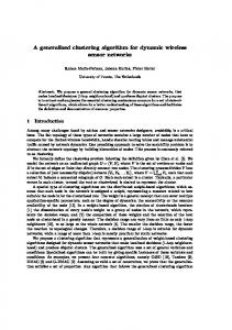
Fig 1: Proposed Architecture of MADCA The proposed architecture describes that the data sensed by the sensor nodes is sent to the sink, where the similarity measure is calculated and the value is given for clustering of nodes. After the nodes are clustered, the sleep duty cycle is generated based on data sending rate and given to the nodes to adaptively enter into sleep/awake state. Also for every clustering period, reclustering is performed by the sink which again proceeds with the similarity measure calculation. In MADCA, the sink node performs all the tasks needed to cluster the sensor network. Those tasks are described in the following four phases: 1. similarity measure calculation, 2. clustering of nodes, 3. generation of sleep-duty cycle, 4. re-clustering for mobile nodes.
3.1 Similarity Measure Calculation In this phase, each sensor node transmits the data to the sink, which in turn gathers the data from the sensor nodes. After collecting enough data, it estimates the similarity measure by
13
International Journal of Computer Applications (0975 – 8887) Volume 20– No.7, April 2011 considering pair of nodes. For finding out the similarity measure, the sink calculates the magnitude of data values of the sensor nodes, distance of the node from the sink and data sending rate. When data is collected continuously, general shape and the trend of the phenomena’s evolving curve are affected as magnitude determines them. Hence, in order to evaluate the similarity of the data, magnitude is taken into consideration. The magnitude of the data is calculated by;
Mi Where
Mi
dvi
is magnitude and
2
dvi
(1) is data value of node
i.
Distance does matter in differentiating the data sensed by the sensors. So it is also taken into consideration in calculating similarity measure of the nodes. The distance of node from sink can be calculated by;
Di Where
Di
x1 ) 2 ( y i 2
( xi 2
is distance, ( xi 2 ,
y1 ) 2
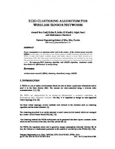
In this phase, sink node uses a clustering algorithm to cluster the sensor nodes by using the similarity measure. The similarity measure of two nodes is compared with the similarity measure threshold and the nodes are clustered using clique-covering algorithm. The input of the clustering algorithm is the graph. The graph is constructed as follows; Each node is considered as a vertex. Edge is drawn between two nodes, if the similarity measure of the two nodes is greater than the similarity measure threshold which is calculated by considering samples. Likewise, similarity measure of all pair wise node is checked out and graph is formed finally. This graph is an input of clustering algorithm. For example, consider the Fig. 2 shown below. The graph contains 5 nodes. It is clear from the graph that similarity measure of node 1 & 2 falls below similarity threshold and similarity measure of 1&3, 1&5, 2&5, 2&4, 5&4 falls above similarity threshold.
(2)
yi 2 ) is coordinates of node i
1
&( 3
x1 , y1 ) is coordinates of sink.
2
Furthermore, data sending rate of the node is used in calculating similarity measure. It is given by;
np
Ri Where
Ri
t
is Data sending rate of node
packets sent and
t
i , np
is number of
is time.
After calculating the magnitude, distance and data sending rate, each node is represented by three dimensions. For example node
i is represented as ( M i , Di , Ri ) and node j as ( M
j , Dj , Rj ) .
5
4
(3)
Fig 2: Example of an Input graph to Clustering The algorithm produces set of clusters as an output. For the graph given in Fig. 2, the number of clusters would be two as shown in Fig. 3.
is represented
nodes is based on these coordinates. In order to estimate the similarity measure between two nodes, Euclidean distance is used. Sink node estimates the similarity measure using the formula:
SM i
3
Cluster 2
2
4
n
( yix
y jx ) 2 , n 3
Cluster 1
1
Similarity Measure (SM) between two
5
(4)
x 1
Where
SM i
Similarity Measure of pair
i
,
y i1
is Magnitude,
y i 2 is Distance and y i 3 is Data sending rate of node 1 in the pair i . y j1
is Magnitude,
y j2
rate of node 2 in the pair
is Distance and
i
y j3
is Data sending
.
3.2 Clustering of Nodes The similarity value calculated in the similarity measure calculation phase is given as an input to the clustering algorithm.
Fig 3: Cluster set of example Input graph After the clusters are formed, in each cluster, the node with highest node degree is chosen as a cluster head. It is important that only few sensor nodes should be active in each cluster at a particular time, in order to save the energy. To accomplish this, it is needed to reduce the number of clusters. So when choosing a similarity measure threshold value, it is taken into consideration, so that the similarity measure threshold which produces minimum number of clusters could be selected. The clique covering algorithm has been given in Fig. 4.
14
International Journal of Computer Applications (0975 – 8887) Volume 20– No.7, April 2011
Clique Covering Algorithm
3.3 Generation of Sleep-Duty Cycle
Input: Graph Gr Output: Cliques Let {uv} be the set of uncovered vertices in the graph Gr , While
{ {uv} Choose
nd (v)
} v {uv} such max{nd (i)} where nd is vertex
degree Let adj(v) be the set of adjacent vertices of
that node
v
adj(v) and put them in {sv} Construct a graph Tgraph = {sv} Sort {sv} in decreasing order of nd ( j ) Construct a clique C {v} While { {sv} } Choose next vertex k {sv} If adj(k ) i i C Pick up
Add
k into C
End if End while Return C Take out the vertices of End while
C
from
Gr
No. of Clusters
25 20
Similarity Threshold Vs No. of Clusters
5 0 0
There are three cases to be considered when generating the sleep-duty cycle. 1.
If data sending rate is lower than minimum rate for some ‘n’ nodes in the cluster, then ‘n’ nodes are put in sleep state.
2.
If data sending rate is greater than minimum rate for all ‘n’ nodes in the cluster, then ‘n/2’ nodes are put in sleep state randomly.
3.
If data sending rate is lower than minimum rate for all ‘n’ nodes in the cluster, then round robin scheduling method is utilized in order to make atleast one node to be awake at the particular time slot.
Then cluster heads take responsibility to collect the data from its members. After collecting the data, the cluster heads process the data and send to the sink. The sink receives the data from the cluster heads. Since the workload is distributed among cluster heads to reduce the overhead of sink, clustering method is called as distributed clustering. If cluster head finds any changes in the value generated and in data sending rate, it informs the sink which in turn updates the schedule once again.
30
10
In order to generate the work schedule, Random Scheduling Method has been adapted. The time needed to find the similarity between two nodes is taken and split into equal size time slots. For each time slot, the sensor nodes within the cluster get into sleep-duty cycle based on their data sending rate and minimum threshold rate.
Once the work schedule is generated, the sink broadcasts the sleep duty cycle information to all sensor nodes with cluster ID, node ID, and sleep wake up time slots. The nodes receive this information and adaptively enter into the energy saving mode according to the schedule.
Fig 4: Clique Covering Algorithm
15
After the clusters are constructed, now it is the time for the sink to generate a sleep-duty cycle for the nodes that are low in data sending rate.
50
Similarity Threshold Fig 5: Similarity Threshold Vs number of Clusters Fig. 5 demonstrates that with the increase of similarity measure threshold, the number of clusters decreases. When number of clusters decreases, the energy saving can be maximized.
3.4 Re-Clustering for Mobile Nodes So far, the algorithm has been formulated for the static nodes. This is the phase, where the algorithm is being updated for the mobile nodes. The static nodes need not be aware of route information as they only communicate with cluster heads and sink. And there is more possibility for the same node to be the cluster head for a long period as nodes are stationary. So the cluster heads may lose their energy so quickly and may die. In the case of mobile nodes, the nodes keep on moving. There are many chances for the change in cluster heads if the algorithm takes care. So the energy utilization is distributed. Though energy utilization is good in mobile nodes, there is a necessity in managing the topology of the network. The location of the nodes changes timely. So the structure of the network cannot be pre-determined. Due to the movement, the path may break at any time. So each node has to have the route information either to communicate with the sink or cluster head. In order to design the algorithm for mobile nodes, the problems associated with mobility are to be analyzed.
15
International Journal of Computer Applications (0975 – 8887) Volume 20– No.7, April 2011 1.
When the nodes are mobile, the path from node to cluster head may get broken, so the node may not be able to reach the cluster head.
2.
The node may move to new location passing the transmission range of its cluster head.
3.
When the cluster heads are mobile, the path from the cluster head to sink may be lost.
4.
Because of the mobility in cluster heads, the packets sent by the nodes might not reach. It will lead to packet loss.
For each cluster Sink checks the data rate
R
If
Rm in
for some
Rm in
Where
Put
On analyzing all these problems, a clustering period
Else if
C p is
introduced. Every clustering period, the sink broadcasts a request message to all the nodes. Once the nodes receive the message from sink, they all send the sensed data to the sink which performs re-clustering. Even though the nodes are moved on to the new location, every clustering period, they are supposed to send the sensed data to the sink not to the cluster heads. And cluster heads also transmit the data to the sink. At the result of re-clustering, the new clusters are formed and new cluster heads are chosen for each cluster. But before the clustering period comes, either the movement of nodes or cluster heads out of the transmission range may cause packet loss. In order to avoid the nodes from waiting for the clustering period, the algorithm is updated as follows; Based on working schedule of nodes, the cluster head sends request to the nodes in the allotted time slot of nodes. Instead of sending the data to the cluster heads, the nodes wait for the request from the cluster heads. After receiving the request, nodes send the data to the cluster heads. If the node does not receive the request from the cluster head in two time slots continuously, it decides that it is non-member of the cluster head and it broadcasts the data. The cluster head that is in the transmission range of the particular node receives and comes to know the arrival of the new node. The cluster head immediately intimates the sink that re-constructs the cluster.
R
'n'
nodes then
is minimum rate and
'n'
Else Put atleast one node in sleep state End If End for Sink broadcasts cluster information and sleep duty cycle End for For each cluster Cluster head sends request to nodes in allotted time slots If node receives the request and sends the data Cluster head collects data and checks If ( R Where SM i
R
Rmin
and
SM i
is
Minimum threshold value of SM i
and
R
) R
values,
SM
values,
R ,
SM tmin
is
.
Send details to sink
Input: Sensed data
End if
Output: Set of clusters
Sink updates the work schedule
For every clustering period
Cp
Else if nodes do not send the data to cluster head
Each sensor node transmits the data to the sink.
Cluster head informs the sink
The sink node receives the data.
Sink re-clusters the network
Sink node estimates the Similarity Measure SM . (By (4))
SM th
SM t min
is Difference between two successive
Rm in
SM
is Difference between two successive
MADCA Algorithm
SM
then
'n / 2' nodes in sleep state
Minimum threshold value of
If
is data rate
nodes in sleep state
Rm in for all nodes 'n' Put
R
where
SM th
Else if node does not receive the request from cluster head Node broadcasts the data
is Similarity Measure
Another cluster head in the radio range receives and informs the sink
threshold
Sink performs re-clustering
Construct a graph End if Output cluster by clique-covering Algorithm
End if End for Fig 6: MADCA Algorithm
16
International Journal of Computer Applications (0975 – 8887) Volume 20– No.7, April 2011 If the cluster head does not receive the data from the node in two time slots continuously, the cluster head decides that the node has moved to an another location. In order to re-cluster the network, the cluster head informs the sink about the change. Thus mobility of nodes is adapted. The MADCA algorithm is given in Fig. 6.
Random way point mobility model has been used to provide mobility to the nodes. It allows mobile nodes to pause in a particular location for some time called pause time. After this time expires, the nodes start to move to random destination based on the speed. The simulation parameters used in the simulation are tabulated in Table 1.
4. PERFORMANCE EVALUATION 4.1 Simulation Setup
4.2 Performance Metrics
The simulation of MADCA is performed in NS2 simulator and the performance is evaluated. In the simulation of MADCA, Mannasim has been used to generate the TCL script easily based on the simulation parameters. For simulating MADCA, a random network deployed in an area 300 x 300m is considered. The number of nodes is varied as 20, 40, 60, 80, 100 and they are deployed randomly over the area. Only one sink is taken and it is placed in the centre of the area. The base station is assumed to be placed 150m away from the area. The transmission range of sink is 150m and the transmission range of nodes is 75m. The initial energy of the sink is 50J and initial energy of nodes is 5J. IEEE 802.11 is used for wireless LANs as the MAC layer protocol. Table 1. Simulation Parameters Parameter name
Values
Area size
300 x 300 m
No. of nodes
20, 40, 60, 80, 100 Channel/Wireless
Channel type Channel MAC
802.11
Link
Link Layer
Physical layer
Mica 2
Antenna
Omni Antenna
Radio propagation
Two Ray Ground
Interface queue and
Drop Tail and 50
Length Simulation time
30sec.
Topology
Random
Pause Time
0.2seconds
Initial energy of nodes
5J
Transmit power
0.036W
Receiving power
0.024W
Sensing power
0.015W
Processing power
0.024W
The performance of MADCA is compared with ADCA [1] which is already proved to be more energy efficient than EEDC [5]. The performance is evaluated in terms of control packet overhead, average end-to-end delay, average delivery ratio and energy consumption. Control Packet Overhead: It is defined as the total number of packets normalized by the total number of received data packets. Average end-to-end Delay: This is the average of overall end-to-end delay from source to destination. Average Packet Delivery Ratio: It is the ratio of total number of packets received and the number of packets sent. Energy Consumption: It is the average energy consumed during transmission, reception, etc.
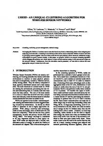
4.3 Simulation Results Based on the number of nodes MADCA is compared with ADCA. The number of nodes varies from 20 to 100. Fig. 7.1, Fig. 7.2, Fig. 7.3 and Fig. 7.4 show the simulation results of both ADCA and MADCA. Both are compared against control overhead, average end-to-end delay, delivery ratio and energy consumption when number of nodes gets increased. Fig. 7.1 shows the control packet overhead generated when applying ADCA and MADCA. The graph demonstrates that the generated overhead packet for MADCA is less than ADCA. When overhead gets reduced, the delay might be minimized and energy could be saved. Fig. 7.2 gives the average end -to- end delay when increasing the number of nodes from 20 to 100. From the graph it is clear that the delay of MADCA is less than ADCA. When delay gets reduced, the energy wastage can be avoided. Fig. 7.3 shows the delivery ratio against the number of nodes. It demonstrates that, in MADCA, the number of packets received successfully is more than the packets received in ADCA. When comparing with the packets sent, MADCA achieves good delivery ratio. Finally, Fig. 7.4 presents the energy spent in both the algorithms. Because of less overhead, reduced delay and good delivery ratio, MADCA is supposed to be more energy efficient. Moreover, as the nodes are mobile, energy consumption by nodes would be less. This is what proved by simulation result and shown in the Fig. 7.4. The simulation results finally say that the algorithm MADCA is more energy efficient than ADCA. ADCA has already been proven to be good in energy efficiency when compared with EEDC. So, energy utilization is far better in MADCA, when evaluating against EEDC and ADCA.
17
4000 3500 3000 2500 2000 1500 1000 500 0
1 0.8
ADCA MADCA
Delivery Ratio
Overhead(No. of Packets)
International Journal of Computer Applications (0975 – 8887) Volume 20– No.7, April 2011
0.6 0.4
ADCA
0.2
MADCA
0 20
20 40 60 80 100
2 1.5 ADCA MADCA
0 40
60
80 100
No. of nodes
Fig 7.2: No. of nodes Vs Delay (Seconds)
5. CONCLUSION In this paper, Mobile Adaptive Distributed Clustering Algorithm has been proposed to minimize the energy consumption in wireless sensor networks. This algorithm is distributed and it reduces the overhead of the sink by clustering the sensor nodes in the network. In order to cluster the network, this algorithm enables the sink to identify the similarity of data among nodes. The nodes that are similar in data are clustered together using clique covering algorithm. In each cluster, the cluster head is chosen. The sleep duty cycle is generated on considering the minimal energy consumption. The changes in the location of nodes are informed to the sink. Besides clustering the network for every clustering period, the sink re-builds the clusters when it receives notification regarding changes in the network. Thus this algorithm helps to lengthen the lifetime of the network. The simulation results have demonstrated that MADCA is better in terms of control overhead, average end-to-end delay, delivery ratio and energy consumption.
Energy Consumption (Joules)
Delay (Seconds)
2.5
20
80 100
Fig 7.3: No. of nodes Vs Delivery ratio
Fig 7.1: No. of nodes Vs Overhead (No. of Packets)
0.5
60
No. of nodes
No. of nodes
1
40
4 3.5 3 2.5 2 1.5 1 0.5 0
ADCA MADCA
20
40
60
80 100
No. of nodes
Fig 7.4: No. of nodes Vs Energy consumption (Joules) MADCA can also be enhanced with more than one sink and the optimal location for placing a sink can also be found, so that the energy can still be reduced further.
6. ACKNOWLEDGMENTS The authors would like to thank all who have supported in bringing out the paper with quality.
7. REFERENCES [1] S.V.Manisekaran, R.Venkatesan, "An Adaptive Distributed Power Efficient Clustering Algorithm for Wireless Sensor Networks", American Journal of Scientific Research, no. 10, pp. 50-63, 2010. [2] Sabitha Ramakrishnan, T.Thyagarajan, "Energy Efficient Medium Access Control for Wireless Sensor Networks", International Journal of Computer Science and Network Security, vol.9, no.6, 2009.
18
International Journal of Computer Applications (0975 – 8887) Volume 20– No.7, April 2011 [3] Mehdi Saeidmanesh, Mojtaba Hajimohammadi, and AliMovaghar, "Energy and Distance Based Clustering: An Energy Efficient Clustering Method for Wireless Sensor Networks", World Academy of Science, Engineering and Technology, vol. 55, p.p 555-559, 2009. [4] Udit, S. and Pabitra, M. 2007. Distributive Energy Efficient Adaptive Clustering Protocol for Wireless Sensor Networks. In Proceedings of the 2007 International Conference on Mobile Data Management, p.p 326-330. [5] Chong Liu, Kui Wu and Jian Pei, "An Energy-Efficient Data Collection Framework", IEEE transactions on parallel and distributed systems, vol. 18, no. 7, p.p 1010-1023, 2007. [6] Nauman Israr, Irfan Awan, "Multihop clustering algorithm for load balancing in wireless sensor networks", International Journal of Simulation, Systems, Science and Technology, 2007. [7] Stanislava, S. and Wendi, B. H. 2005. Prolonging the Lifetime of Wireless Sensor Networks via Unequal Clustering. In Proceedings of the 19th IEEE International Parallel and Distributed Processing Symposium, p.p 8-16. [8] Ossama Younis, Sonia Fahmy, "HEED: A Hybrid Energy - Efficient, Distributed Clustering Approach for Ad-hoc Sensor Networks", IEEE Transactions on Mobile Computing, vol.3, no. 4, p.p 366 – 379, 2004. [9] Pavlos, P. 2002. Literature Survey on Wireless Sensor Networks, In Proceedings of the First ACM International Workshop on Wireless Sensor Networks and Applications. [10] Wendi, R.H., Anantha, C. and Hari, B. 2000. EnergyEfficient Communication Protocol for Wireless
Microsensor Networks. In Proceedings of the 33rd Hawaii International Conference on System Sciences.
AUTHORS PROFILE S.V.Manisekaran was born in Tamilnadu, India in 1981. He received his B.E. degree in Information Technology from Bharathiyar University, Coimbatore in 2003. He completed his M.E. in Computer Science and Engineering from Anna University Chennai in 2005. He is currently working as an Assistant Professor in the Department of Information Technology at Anna University of Technology, Coimbatore, India. His research areas include mobile computing, quality management and software engineering. R.Venkatesan was born in Tamilnadu, India, in 1958. He received his B.E (Hons) degree from Madras University in 1980. He completed his Masters degree in Industrial Engineering from Madras University in 1982. He obtained his second Masters degree MS in Computer and Information Science from University of Michigan, USA in 1999. He was awarded with PhD from Anna University, Chennai in 2007. He is currently Professor and Head in the Department of Computer Science and Engineering at PSG College of Technology, Coimbatore, India. His research interests are in Simulation and Modeling, Software Engineering, Algorithm Design, Software Process Management. G. Deivanai was born in Tamilnadu, India, in 1983. She received her B.Tech degree in Information Technology from Anna University, Chennai in 2005. She is currently pursuing her M.Tech in Information Technology at Anna University of Technology, Coimbatore. Her areas of interests include wireless network, wireless sensor network and middleware technologies.
19