Model-Based Learning of Turbulent Flows using Mobile Robots

1

Model-Based Learning of Turbulent Flows using Mobile Robots

arXiv:1812.03894v1 [cs.RO] 10 Dec 2018

Reza Khodayi-mehr, Student Member, IEEE and Michael M. Zavlanos, Member, IEEE

Abstract—In this paper we consider the problem of modelbased learning of turbulent flows using mobile robots. The key idea is to use empirical data to improve on numerical estimates of time-averaged flow properties that can be obtained using Reynolds-Averaged Navier Stokes (RANS) models. RANS models are computationally efficient and provide global knowledge of the flow but they also rely on simplifying assumptions and require experimental validation. In this paper, we instead construct statistical models of the flow properties using Gaussian Processes (GPs) and rely on the numerical solutions obtained from RANS models to inform their mean. We then utilize Bayesian inference to incorporate empirical measurements of the flow into these GPs, specifically, measurements of the time-averaged velocity and turbulent intensity fields. Our formulation accounts for model ambiguity and parameter uncertainty via hierarchical model selection. Moreover, it accounts for measurement noise by systematically incorporating it in the GP models. To obtain the velocity and turbulent intensity measurements, we design a cost-effective mobile robot sensor that collects and analyzes instantaneous velocity readings. We control this mobile robot through a sequence of waypoints that maximize the information content of the corresponding measurements. The end result is a posterior distribution of the flow field that better approximates the real flow and also quantifies the uncertainty in the flow properties. We present experimental results that demonstrate considerable improvement in the prediction of the flow properties compared to pure numerical simulations. Index Terms—Model-based Learning, Active Sensing, Mobile Sensors, Gaussian Processes, Turbulent Flow.

I. I NTRODUCTION Knowledge of turbulent flow properties, e.g., velocity and turbulent intensity, is of paramount importance for many engineering applications. At larger scales, these properties are used for the study of ocean currents and their effects on aquatic life, [1], [2], [3], meteorology, [4], bathymetry, [5], and localization of atmospheric pollutants, [6], to name a few. At smaller scales, knowledge of flow fields is important in applications ranging from optimal HVAC of residential buildings for human comfort, [7], to design of drag-efficient bodies in aerospace and automotive industries, [8]. At even smaller scales, the characteristics of velocity fluctuations in vessels are important for vascular pathology and diagnosis, [9] or for the control of bacteria-inspired uniflagellar robots, [10]. Another important application that requires global knowledge of the velocity field is chemical source identification in advection-diffusion transport systems, [11], [12], [13]. Reza Khodayi-mehr and Michael M. Zavlanos are with the Department of Mechanical Engineering and Materials Science, Duke University, Durham, NC 27708, USA, {reza.khodayi.mehr, michael.zavlanos}@duke.edu.

The most cost-effective way to estimate a flow field is using numerical simulation and the Navier-Stokes (NS) equations. These equations are a set of Partial Differential Equations (PDEs) derived from first principles, i.e., conservation of mass, momentum, and energy, that describe the relationship between flow properties, [14]. They can be simplified depending on the nature of the flow, e.g., laminar versus turbulent or incompressible versus compressible, to yield simpler, more manageable equations. Nevertheless, when the flow is turbulent, solving the NS equations becomes very challenging due to the various time and length scales that are present in the problem. Turbulent flow is characterized by random fluctuations in the flow properties and is identified by high Reynolds numbers. In many of the applications discussed before, especially when air is the fluid of interest, even for very small velocities the flow is turbulent. In this case, Direct Numerical Solution (DNS) of the NS equations is still limited to simple problems. A more effective approach is to solve the time-averaged models called Reynolds-Averaged Navier Stokes equations, or RANS for short. RANS models are useful since in many engineering applications we are interested in averaged properties of the flow, e.g., the mean velocity components, and not the instantaneous fluctuations. Note that despite its chaotic nature, turbulent flow has structure; it consists of eddies that are responsible for generation and dissipation of kinetic energy in a cascade that begins in large or integral scales and is dissipated to heat in small scales called Kolmogorov scales. Understanding these structures is essential for proper modeling of turbulence; see [15] for more details. Averaging the flow properties in RANS models introduces additional unknowns, called Reynolds stresses, in the momentum equation that require proper modeling to complete the set of equations that are solved. This is known as the ‘closure problem’. Depending on how this problem is addressed, various RANS models exist that are categorized into two large classes, Eddy Viscosity Models (EVMs) and Reynolds Stress Models (RSMs); see [15] for more details. The former assume that the Reynolds stress is proportional to the strain defining, in this way, an effective turbulent viscosity, while in the latter a transport equation is derived for the Reynolds stress components and is solved together with the averaged flow equations. EVMs have an assumption of isotropy builtinto them meaning that the Reynolds stresses are directionindependent. Although this assumption is not valid for flow fields that have strong asymmetries, there are many benchmark problems for which the results from EVMs are in better agreement with empirical data than RSMs; see e.g. [16]. In general, solutions provided by these RANS models are not necessarily

2

compatible with each other and more importantly with the real world and require experimental validation, [17]. Furthermore, precise knowledge of the Boundary Conditions (BCs) and domain geometry is often unavailable which contributes to even more inaccuracy in the predicted flow properties. Finally, appropriate meshing is necessary to properly capture the boundary layer and get convergent solutions from RANS models, which is not a straight-forward process. In order to address the shortcomings of RANS models and complement the associated numerical methods, various experimental techniques have been developed that directly measure the flow properties. These methods can also be used as stand-alone approaches alleviating the need for accurate knowledge of the BCs and geometry. A first approach of this kind utilizes hot-wire constant temperature anemometers. A hot-wire anemometer is a very thin wire that is placed in the flow and can measure flow fluctuations up to very high frequencies. The fluctuations are directly related to the heat transfer rate from the wire, [18]. Hot-wire sensors are very cost effective but require placing equipment in the flow that might interfere with the pattern and is not always possible. A next generation of approaches are optical methods that seed particles in the flow and optically track them. Two of the most important variants of optical methods are Particle Imaging Velocimetry (PIV) and Laser-Doppler Anemometry (LDA). In PIV, two consecutive snapshots of the particles in the flow are obtained and their spatial correlation is used to determine the shift and the velocity field, [19]. On the other hand, in LDA a pair of intersecting beams create a fringe in the desired measurement location. The light from a particle passing through this fringe pulsates and the frequency of this pulse together with the fringe spacing determine the flow speed, [20]. Optical methods although non-intrusive, require seeding particles with proper density and are expensive. Another sensing approach utilizes Microelectromechanical Systems (MEMS) for flow measurements. Because of their extremely small size and low cost, these devices are a very attractive alternative to aforementioned methods, [21]. Empirical data from experiments are prone to noise and error and are not always available for various reasons, e.g., cost and accessibility, scale of the domain, and environmental conditions. On the other hand, as discussed before, numerical simulations are inaccurate and require validation but are costeffective and can provide global information over the whole domain. In this paper we propose a model-based learning method that combines numerical solutions with empirical data to improve on the estimation accuracy of flow properties. Specifically, we construct a statistical model of the timeaveraged flow properties using Gaussian Processes (GPs) and employ the physics of the problem, captured by RANS models, to inform their prior mean. We construct GPs for different RANS models and realizations of the random BCs and other uncertain parameters. We also derive expressions for measurement noise and systematically incorporate it into our GP models. To collect the empirical data, we use a custom-built mobile robot sensor that collects and analyzes instantaneous velocity readings and extracts time-averaged velocity and turbulent intensity measurements. Specifically,

we propose an online path planning method that guides the robot through optimal measurement locations that maximize the amount of information collected about the flow field. Then, using Bayesian inference and hierarchical model selection, we obtain the posterior probabilities of the GPs and the flow properties for each model after conditioning on the empirical data. The proposed robotic approach to learning the properties of turbulent flows allows for fewer, more informative measurements to be collected. Therefore, it is more efficient, autonomous, and can be used for learning in inaccessible domains. II. R ELATED W ORK A. Machine Learning in Fluid Dynamics Machine Learning (ML) algorithms have been used to help characterize flow fields. One way to do this is by model reduction, which speeds up the numerical solutions, [22], [23], [24], [25]. Particularly, [22] utilizes Neural Networks to reduce the order of the physical model and introduce a correction term in the Taylor expansion of the near wall equations that improves the approximations considerably. [23] uses Deep Learning to construct an efficient, stable, approximate projection operator that replaces the iterative solver needed in the numerical solution of the NS equations. [24] proposes an alternative approach to traditional numerical methods utilizing a regression forest to predict the behavior of fluid particles over time. The features for the regression problem are selected by simulating the NS equations. A different class of methods utilize ML to improve accuracy instead of speed. For instance, [26] presents a modification term in the closure model of the RANS equations which is learned through data collected experimentally or using DNSs. The modified closure model replaces the original one in the RANS solvers. In a different approach, [17] utilizes classification algorithms to detect regions in which the assumptions of the RANS models are violated. They consider three of the main underlying assumptions: (i) the isotropy of the eddy viscosity, (ii) the linearity of the Boussinesq hypothesis, and (iii) the nonnegativity of the eddy viscosity. The approaches discussed above mainly focus on application of ML to improve on the speed or accuracy of the RANS models at the solver level without considering various sources of uncertainty that are not captured in these models, e.g., imperfect knowledge of the BCs and geometry. To the contrary, here we focus on validation, selection, and modification of the solutions obtained from RANS models using a datadriven approach. Particularly, we employ Gaussain Processes (GPs) to model the flow field and propose a supervised learning strategy to incorporate empirical data into numerical RANS solutions in real-time. GPs provide a natural way to incorporate measurements into numerical solutions and to construct posterior distributions in closed-form. Note that GPs have been previously used to model turbulent flows in other contexts. For instance, [26] uses GPs to modify closure models and improve accuracy while [27] models turbulent fields via GPs and then use these GPs to obtain probabilistic models for the dispersion of particles in the flow field. Since turbulence is

3

a non-Gaussian phenomenon, assuming Gaussianity is a major approximation, [28]. Nevertheless, here we focus on mean flow properties which are Normally distributed regardless of the underlying distribution of the instantaneous properties, [29].

PDEs. Solutions to the NS equations depend on uncertain parameters like BCs and geometry. We propose a model-based approach to learn the posterior distributions of these solutions along with the flow properties.

B. Active Learning for Gaussian Processes

C. Contributions

Active learning using GPs has been investigated extensively in the robotics literature. This is because of the closed form of the posterior distribution that makes GPs ideal for inference and planning. Collecting informative data in active learning applications depends on defining appropriate optimality indices for planning with entropy and Mutual Information (MI) being the most popular ones. Particularly, MI is submodular and monotone and can be optimized using greedy approaches while ensuring sub-optimality lower-bounds; see [30]. Necessary conditions to obtain such sub-optimality lower bounds for MI are discussed in [31]. When used for planning, such optimality indices can guide mobile robots through sequences of measurements with maximum information content. For example, [32] proposes a suboptimal, non-greedy trajectory planning method for a GP using MI, while [2] relies on Markov Decision Processes and MI to plan paths for autonomous under-water vehicles. On the other hand, [33] collects measurements at the next most uncertain location which is equivalent to optimizing the entropy. In this paper, we employ a similar approach where the mobile sensor plans its path to minimize the entropy of unobserved areas in the flow. Active learning using GPs has applications ranging from estimation of nonlinear dynamics to spatiotemporal fields. For instance, [33] presents an active learning approach to determine the region of attraction of a nonlinear dynamical system. The authors decompose the unknown dynamics into a known mean and an unknown perturbation which is modeled using a GP. Also, [34], [35] use similar approaches to estimate and control nonlinear dynamics using robust and model predictive control, respectively. [36] presents an active sensing approach using cameras to associate targets with their corresponding nonlinear dynamics where the target behaviors are modeled by Dirichlet process-GPs. On the other hand, [1] uses GPs to estimate the uncertainty in predictive ocean current models and rely on the resulting confidence measures to plan the path of an autonomous under-water vehicle. GPs have also been used for estimation of spatiotemporal fields, e.g., velocity and temperature. For instance, [37] proposes a learning strategy based on subspace identification to learn the eigenvalues of a linear time-invariant dynamic system which defines the temporal evolution of a field. [38] addresses the problem of trajectory planning for a mobile sensor to estimate the state of a GP using a Kalman filter. Closely related are also methods for robotic state estimation and planning with Gaussian noise; see [39], [40], [41]. The literature discussed above typically employs simple, explicit models of small dimensions and does not consider model ambiguity or parameter uncertainty. Instead, here we consider much more complex models of continuous flow fields that are implicit solutions of the NS equations, a system of

The contributions of this work can be summarized as follows: (i) To the best of our knowledge, this is the first model-based framework that can be used to learn flow fields using empirical data. To this date, ML methods have only been used to speed up numerical simulations using RANS models or to increase their accuracy. Instead, the proposed framework learns solutions of the NS equations by combining theoretical models and empirical data in a way that allows for validation, selection, and more accurate prediction of the flow properties. Compared to empirical methods to estimate flow fields, this is the first time that robots are used for data collection, while compared to relevant active learning methods in robotics, the flow models we consider here are much more complex, uncertain, and contain ambiguities that can only be resolved using empirical validation. (ii) We design a costeffective flow sensor mounted on a custom-built mobile robot that collects and analyzes instantaneous velocity readings. We also propose a planning algorithm for the mobile robot based on the entropy optimality index to collect measurements with maximum information content and show that it outperforms similar planning methods that possess sub-optimality bounds. (iii) The proposed framework is able to select the most accurate models, obtain the posterior distribution of the flow properties and, most importantly, predict these properties at new locations with reasonable uncertainty bounds. We experimentally demonstrate the predictive ability of the posterior field and show that it outperforms prior numerical solutions. The remainder of the paper is organized as follows. In Section III, we discuss properties of turbulent flows and develop a statistical model to capture the velocity field and corresponding turbulent intensity. Section IV describes the design of the mobile sensor, the proposed algorithms to collect and process the instantaneous velocity readings, the formulation of the measurement errors, and finally the proposed planning method for the mobile sensor to collect flow measurements. In Section V, we present experiments that demonstrate the ability of the posterior field to better predict the flow properties at unobserved locations. Finally, Section VI concludes the paper. III. S TATISTICAL M ODEL OF T URBULENT F LOWS In this section, we discuss the theoretical aspects of turbulence that are needed to model the flow field. We also present a statistical model of turbulent flows and discuss its components. A. Reynolds-Averaged Navier Stokes Models Since turbulence is a 3D phenomenon, consider a 3D ¯ ⊂ R3 and the velocity vector field domain of interest Ω ¯ q(t, x) : [t0 , tf ] × Ω → R3 defined over this domain where ¯ Following the analysis used in RANS t ∈ [t0 , tf ] and x ∈ Ω.

4

models, we decompose the velocity field into its time-averaged value and a perturbation as q(x, t) = q(x) + (x, t),

(1)

where 1 q(x) = lim T →∞ T

Z

t1 +T

q(x, t)dt. t1

In order for this limit to exist, we assume that the flow is ‘stationary’ or ‘statistically steady’. Under this condition, the integral will be independent of t1 . Since turbulent flows are inherently random, we can view q(x, t) or equivalently (x, t) as a Random Vector (RV). Let qj (x, t) denote j-th realization of this RV at location x and time t and consider the ensemble average defined as n ˆ

ˆ (x, t) = q

1X j q (x, t), n ˆ j=1

where n ˆ is the total number of realizations. Assuming ‘ergodˆ (t, x) is independent of time so that q ˆ (t, x) = q(x). icity’, q This is a common assumption that allows us to obtain timeseries measurements of the velocity field at a given location and use the time-averaged velocity q(x) as a surrogate for the ˆ (x, t). ensemble average q Next, consider the Root Mean Square (RMS) value of the fluctuations of the k-th velocity component defined as !0.5 Z 1 t1 +T 2 |k (x, t)| dt . qk,rms (x) = lim T →∞ T t 1 Noting that (x, t) = q(x, t) − q(x) and using the ergodicity assumption, we have 2

ˆ k (x, t)] = q2k,rms (x), var[qk (x, t)] , E [qk (x, t) − q where var[·] denotes the variance of a Random Variable (RV). The average normalized RMS value is called turbulent intensity and is defined as i(x) =

kqrms (x)k √ , 3 qref

(2)

where qref is the normalizing velocity. This value is an isotropic measure of the average fluctuations caused by turbulence at point x. Finally, we consider the integral time scale t∗k (x) of the turbulent field along the k-th velocity direction, defined as Z ∞ 1 t∗k (x) = ρk (τ ) dτ, (3) ρk (0) 0 where ρk (τ ) is the autocorrelation of the velocity given by Z 1 T ρk (τ ) = lim k (x, t) k (x, t + τ )dt, T →∞ T 0 and τ is the autocorrelation lag. We use the integral time scale to determine the sampling frequency in Section III-C3. For more details on turbulence theory, see [15].

B. Statistical Flow Model The RANS models use the decomposition given in (1) to obtain turbulence models for the mean flow properties. As discussed in Section I, depending on how they address the closure problem, various RANS models exist. The numerical results returned by these models depend on the geometry of the domain, the values of the Boundary Conditions (BCs), and the model that is used, among other things. Since there is high uncertainty in modeling the geometry and BCs and since the RANS models may return inconsistent solutions, numerical methods often require experimental validation. On the other hand, empirical data is prone to noise and this uncertainty needs to be considered before deciding on a model that best matches the real flow field. Bayesian inference provides a natural approach to combine theoretical and empirical knowledge in a systematic manner. In this paper, we utilize Gaussian Processes (GPs) to model uncertain flow fileds; see [42]. Using GPs and Bayesian inference we can derive the posterior distributions of the flow parameters conditioned on available data in closed-form. Note that while turbulence is a nonGaussian phenomenon, [28], the time-averaged velocity and turbulent intensity fields are Normally distributed regardless of the underlying distribution of the instantaneous velocity field. Therefore, we define GP models for these time-averaged quantities, whose knowledge happens to also be the most important for many engineering applications. We construct the proposed GP models based on numerical solutions as opposed to purely statistical models, i.e., empirical data are used only to modify model-based solutions and not to replace them. Particularly, given a mean function µ(x) and a kernel function κ(x, x0 ), we denote a GP by GP(µ(x), κ ¯ (x, x0 )). The mean function is given by the numerical solution from a RANS model and we define the kernel function as κ ¯ (x, x0 ) = σ ¯ 2 (x, x0 )ρ(x, x0 ),

(4)

where σ ¯ (x, x0 ) encapsulates the uncertainty of the field and 0 ρ(x, x ) is the correlation function. Here we define this function as a compactly supported polynomial 2  kx − x0 k , (5) ρ(x, x0 ) = 1 − ` + where ` ∈ R+ is the correlation characteristic length and we define the operator (α)+ = max(0, α). The correlation function (5) implies that, two points with distance larger than ` are uncorrelated, which results in a sparse covariance matrix. In the following we use a constant standard deviation, i.e., we set σ ¯ (x, x0 ) = σ ¯. Consider a measurement model with additive Gaussian noise  ∼ N (0, σ 2 (x)) and let y(x) ∈ R denote a measurement at location x given by y(x) = GP(µ(x), κ ¯ (x, x0 )) + (x). Then y(x) is also a GP y(x) ∼ GP(µ(x), κ(x, x0 ))

(6)

5

with the following kernel function 0

0

2

0

κ(x, x ) = κ ¯ (x, x ) + σ (x) δ(x − x ),

(7)

where δ(x − x0 ) is the Dirac delta function. Given a vector of measurements y at a set of locations X , we can obtain the conditional distribution of (6) at a point x which is a Gaussian distribution N (µ, γ 2 ) with mean and variance given by µ(x|X ) 2

γ (x|X )

= µ(x) + ΣxX Σ−1 X X (y − µX ) , = κ ¯ (x, x) −

ΣxX Σ−1 X X ΣX x ,

(8a)

for u(x), with mean µu (x) obtained from the numerical solution of a RANS model and the standard deviation in (4) defined as σ ¯u (x, x0 ) = σ ¯u . This value is a measure of confidence in the numerical solution µu (x) and can be adjusted to reflect this confidence depending on the model that is utilized and the convergence metrics provided by the RANS solver. GPs for the other velocity components v and w can be defined in a similar way. On the other hand, denoting by i(x) the turbulent intensity at point x, we can define a GP (10)

for i(x), where, as before, we select the prior mean µi (x) from the numerical solution of a RANS model and define the standard deviation in the kernel function (4) by a constant, i.e., σ ¯i (x, x0 ) = σ ¯i . C. Measurement Model Next, we discuss equation (6) used to obtain measurements of the velocity components and turbulent intensity. Specifically, at a given point x, we collect a set of instantaneous velocity readings over a period of time and calculate the sample mean and variance. Note that by the ergodicity assumption, these time samples are equivalent to multiple realizations of the RV q(x, t); see Section III-A. 1) Mean Velocity Components:: Consider the instantaneous first component of the velocity u(x, t) and a sensor model that has additive noise with standard deviation γu,s (x, t) ∈ R+ . An observation yu (x, t) of this velocity at a given point x and time t is given by yu (x, t) = u(x, t) + u,s (x, t),

(11)

2 N (0, γu,s )

where u,s (x, t) ∼ is the instantaneous measurement noise. Assume that we collect n uncorrelated samples of yu (x, t) at time instances tk for 1 ≤ k ≤ n. Then, the sample mean of the first velocity component is given by n

yu (x) =

1X yu (x, tk ) n k=1

var[yu (x)] =

n 1 X 1 var[yu (x, t)] = var[yu (x, t)]. n2 n

(12)

(13)

k=1

An unbiased estimator of var[yu (x, t)] is the sample variance

(8b)

where µX denotes the mean function evaluated at measurement locations X and the entries of the covariance matrices ΣxX and ΣX X are computed using (7). The GPs discussed above are defined individually for each one of the flow properties of interest, i.e., the 3D velocity field and the turbulent intensity. Specifically, denoting by u(x) the first mean velocity component at point x, we can define the GP u(x) ∼ GP(µu (x), κu (x, x0 )) (9)

i(x) ∼ GP(µi (x), κi (x, x0 )),

and is a random realization of the mean first velocity component u(x). Since the samples yu (x, tk ) are uncorrelated, the variance of yu (x) is given by

n

var[y ˆ u (x, t)] =

1 X 2 [yu (x, tk ) − yu (x)] . n−1

(14)

k=1

Substituting this estimator in (13), we get an estimator for the variance of yu (x) as n

var[y ˆ u (x)] =

X 1 2 [yu (x, tk ) − yu (x)] . n (n − 1)

(15)

k=1

Note that as we increase the number of samples n, yu (x) becomes a more accurate estimator of u(x). Given the observation yu (x), we construct the measurement model for the mean first component of the velocity as yu (x) = u(x) + u (x),

(16)

where u (x) is the perturbation with variance σu2 (x); cf. equation (7). Note that the distribution of yu (x) is Gaussian as long as the measurement noise u,s (x, t) in (11) is Gaussian; see [29]. In Section IV-B, we show that for typical off-theshelf sensors, a Gaussian model is a good approximation for the measurement noise. Note that in addition to sensor noise 2 , captured in the sample mean variance (14), other sources γu,s of uncertainty may contribute to σu2 (x). In Section IV-B, we derive an estimator for this variance taking into account these additional sources of uncertainty. Next, we take a closer look at var[yu (x, t)] and the terms that contribute to it. Since the variance of the sum of uncorrelated RVs is the sum of their variances, from (11) we get 2 var[yu (x, t)] = var[u(x, t)] + γu,s (x, t). Furthermore, since the samples yu (x, tk ) are uncorrelated, we have n X

var[yu (x, tk )] =

k=1

n X 

2 var[u(x, tk )] + γu,s (x, tk ) ,

k=1

and thus, 2 var[yu (x, t)] = var[u(x, t)] + γ¯u,s (x),

where

(17)

n

2 γ¯u,s (x) =

1X 2 γu,s (x, tk ) n

(18)

k=1

is the mean variance of the sensor noise. We derive an 2 expression for the instantaneous variance γu,s (x, tk ) in Section IV-B. Notice from equation (17) that the variance of yu (x, t) is due to turbulent fluctuations and sensor noise u,s (x, t). The former is a variation caused by turbulence and inherent to the RV u(x) whereas the latter is due to inaccuracy in sensors and further contributes to the uncertainty of the mean velocity component u(x).

6

2) Turbulent Intensity:: Referring to (2), turbulent intensity at a point x is given as !0.5 3 X 2 i(x) ∝ kqrms (x)k = . qk,rms (x)

In practice, we only have a finite set of samples of the instantaneous velocity vector over time and can only approximate (3). Let l denote the discrete lag. Then, the sample autocorrelation of first velocity component is n−l

k=1

Note that by the ergodicity assumption q21,rms (x) = var[u(x, t)] and similarly for the other velocity components; see Section III-A. Then, using equations (17) and (14), we have 2 2 ˆi(x) = √ 1 var[y ˆ u ] − γ¯u,s (x) + var[y ˆ v ] − γ¯v,s (x) 3 qref
0.5 2 , (19) +var[y ˆ w ] − γ¯w,s (x) where variances of the instantaneous velocity measurements var[y ˆ v (x, t)] and var[y ˆ w (x, t)] and the corresponding mean 2 2 (x) are computed using sensor noise variances γ¯v,s (x) and γ¯w,s equations similar to (14) and (18), respectively. Let i (x) ∼ N (0, σi2 ) denote the error in the turbulent intensity estimate. Then, we define the corresponding measurement yi (x) = ˆi(x) as yi (x) = i(x) + i (x).

(20)

Note that, unlike the mean velocity measurements, it is not straight-forward to theoretically obtain the variance of the turbulent intensity measurement. This is due to the nonlinearity in definition (2). In general, estimating this variance requires the knowledge of higher order moments of the random velocity components; cf. [29]. Specifically under a Gaussianity assumption, they depend on the mean values yu (x), yv (x) and yw (x) which are not necessarily negligible. Consequently, we need to incorporate this uncertainty into our statistical model. Here, we utilize the Bootstrap resampling method to directly estimate the variance σi2 . Assume that the samples yu (x, tk ) are independent and consider the measurement set Yu = {yu (x, tk ) | 1 ≤ k ≤ n}; define Yv and Yw similarly. Furthermore, consider nb batches Bj of size n obtained by randomly drawing the same samples from Yu , Yv , and Yw with replacement. Using (19), we obtain nb estimates ˆij (x) corresponding to the batches Bj . Then, the desired variance σi2 (x) can be estimated as b 1 X = (ˆij − ¯i)2 , nb − 1 j=1

1X [yu (x, tk ) − yu (x)][yu (x, tk+l ) − yu (x)]. n k=1

This approximation becomes less accurate as l increases since the number of samples used to calculate the summation decreases. Furthermore, the integral of the sample autocorrelation ρˆu (l) over the range 1 ≤ l ≤ n − 1 is constant and equal to 0.5; see [44]. This means that we cannot directly use (3) which requires integration over the whole time range. The most common approach is to integrate ρˆu up to the first zerocrossing; see [45]. D. Hierarchical Model Selection Thus far, we have assumed that a single numerical solution is used to obtain the proposed statistical model. In this section, we show how to incorporate multiple numerical solutions in this statistical model. This is necessary since different RANS models may yield different and even contradictory approximations of the flow field. This effect is exacerbated by the uncertainty in the parameters contained in RANS models; see Section I. On the other hand, incorporating solutions from multiple RANS models in the proposed statistical model of the flow allows for a better informed prior mean and ultimately for model selection and validation using empirical data. Specifically, consider a RV that collects all secondary variables that affect the numerical solution including uncertain BCs. Given an arbitrary distribution for each variable, we can construct a discrete distribution that approximates the continuous distributions using, e.g., a Stochastic Reduced Order Model (SROM); cf. [46] for details. Let Mj denote the j-th numerical solution corresponding to one combination n ¯ of all these RVs and let the collection π ˜ (Mj ) = {pj , Mj }j=1 denote the discrete distribution, where n ¯ is the number of discrete models. Given a vector of measurements yk at a set of locations Xk , the posterior distribution over these discrete models can be easily obtained using Bayes’ rule as π ˜ (Mj |Xk ) = α π ¯ (yk |Mj ) π ˜ (Mj ),

n

σ ˆi2 (x)

ρˆu (l) =

(21)

where ¯i(x) is the mean of batch estimates ˆij (x); see [43] for more details. 3) Sampling Frequency:: In the preceding analysis, a key assumption was that the samples are independent. Since fluid particles cannot have unbounded acceleration, their velocities vary continuously and thus consecutive samples are dependent. As a general rule of thumb, in order for the samples to be independent, the interval between consecutive sample times tk and tk+1 must be larger than 2 t∗ (x) where t∗ (x) = max t∗k (x), k

is the maximum of the integral time scales (3) along different velocity directions k at point x.

(22)

where α is the normalizing constant and π ¯ (yk |Mj ) is the likelihood of the data given model Mj . Note that we have the marginal distributions π ¯ (yk |Mj ) in closed-form from the definition of the GP as π ¯ (yk |Mj ) = det(2π Σj )−0.5   1 T −1 exp − (yk − µj ) Σj (yk − µj ) , 2 where µj and Σj are short-hand notation for the mean and covariance of the GP constructed using P model Mj , see the n ¯ discussion after equation (8). Noting that k=1 π ˜ (Mj |Xk ) = 1, we compute α as  −1 n ¯ X α= π ¯ (yk |Mj ) π ˜ (Mj ) . (23) j=1

7

µu (x|Xk ) =

n ¯ X

pj,k µu (x|Xk , Mj ),

(24a)

j=1

γu2 (x|Xk ) = +

n ¯ X j=1 n ¯ X

1

0.8

0.6

velocity (m/s)

Given α, we can easily compute the posterior distribution π ˜ (Mj |Xk ) over the discrete models. Then, the desired mean velocity component fields and the turbulent intensity field are the marginal distributions π(u|Xk ), π(v|Xk ), π(w|Xk ), and π(i|Xk ) after integrating over the discrete models. These marginal distributions are GP mixtures with their mean and variance given by

experiment theoretical prediction maximum measurement angle maximum detection angle

0.4

0.2

pj,k γu2 (x|Xk , Mj )

(24b) 0

2

pj,k [µu (x|Xk , Mj ) − µu (x|Xk )] ,

j=1

where pj,k = π ˜ (Mj |Xk ) denotes the posterior model probabilities obtained from (22). Equation (24b) follows from the principal that the variance of a RV is the mean of conditional variances plus the variance of the conditional means. The expressions for v(x), w(x), and i(x) are identical. IV. L EARNING F LOW F IELDS USING M OBILE ROBOT S ENSORS

-0.2 -40

-20

0

20

40

60

80

angle (degrees)

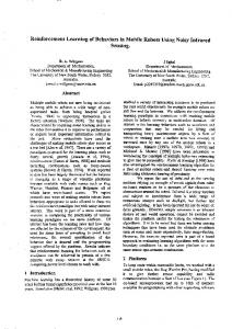
Fig. 1: Directivity plot of the flow sensor used in the mobile robot where we measure the angle from the axis of the sensor. Above 55o the measurements deviate from the theoretical prediction and above 75o there is no detection. The bars on the experimental data show the standard deviation of the sensor samples caused by turbulent fluctuations and sensor noise.

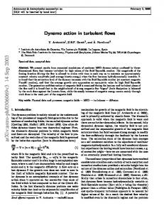
In the previous section, we proposed a statistical model of turbulent flows based on GPs. Next, we develop a mobile robot sensor to measure the instantaneous velocity vector and extract the necessary measurements discussed in Section III-C. We also characterize the uncertainty associated with collecting these measurements by a mobile robot and formulate a path planning problem for it to maximize the information content of these measurements. A. Mobile Sensor Design For simplicity, in what follows we focus on the in-plane components of the velocity field and take measurements on a plane parallel to the ground. Extension to the 3D case is straightforward. Particularly, we use the D6F-W01A1 flow sensor from OMRON; see Section V for more details. Figure 1 shows the directivity pattern for this sensor measured empirically. In this figure, the normal velocity component q cos θˆ is given as a function of the velocity magnitude q and the angle θˆ of the flow from the axis of the sensor. It can be seen that there exists an angle above which the measurements deviate from the mathematical formula and for an even larger angle, no flow is detected at all. The numerical values for these angles are roughly 55o and 75o for the sensor used here. This directivity pattern can be used to determine the maximum angle spacing between sensors mounted on a plane perpendicular to the robot’s z-axis, so that any velocity vector on the x − y plane can be measured accurately. This spacing is 45o , which means that eight sensors are sufficient to sweep the plane. Figure 2 shows the mobile sensor comprised of these eight sensors separated by 45o giving rise to a sensor rig that can completely cover the flow in the plane of measurements. In this configuration, one sensor in the rig will have the highest

Fig. 2: Structure of the mobile sensor and arrangement of the flow velocity sensors. Eight sensors are placed in two rows in the center of the robot with an angle spacing of 90o in each row and combined spacing of 45o .

reading at a given time t with one of its neighboring sensors having the next highest reading. Let q and θ denote the magnitude and angle of the instantaneous flow vector and sj and βj denote the j-th sensor’s reading and heading angle in the global coordinate system where 1 ≤ j ≤ 8. Assume that

8

Algorithm 1 Flow Measurements using Mobile Sensor Require: Measurement location x, sample number n, and the orientation β of the mobile sensor; 1: Given β, compute sensor headings βj for 1 ≤ j ≤ 8; 2: for k = 1 : n do 3: Receive the readings s ∈ R8 from all sensors; 4: Let j and l denote sensors with the highest readings; 5: if |j − l| > 1 then 6: warning: inaccurate sample! 7: end if 8: Let ξ = sign[sin(βj − βl )] and compute: θ = arctan[ξ(sj cos βl − sl cos βj ), ξ(−sj sin βl + sl sin βj )]. 9: 10: 11: 12: 13: 14: 15: 16: 17: 18: 19: 20: 21:

if θ < min {βj , βl } or max {βj , βl } < θ then warning: inaccurate sample! end if Velocity magnitude: q = sj / cos(θ − βj ); ˆ u,k = q cos θ; First velocity component: y ˆ v,k = q sin θ; Second velocity component: y end for First mean velocity component: yu = mean(ˆ yu ); Second mean velocity component: yv = mean(ˆ yv ); ˆv2 via (34) and (37); Compute sample variances σ ˆu2 and σ Compute turbulent intensity measurement yi via (19); Compute variance σ ˆi2 of turbulent intensity using (21); Return yu , yv , yi , σ ˆu2 , σ ˆv2 , and σ ˆi2 ;

sensors j and l have the two highest readings. Then, we have sj = q cos(θ − βj ) and sl = q cos(θ − βl ) ⇒ (25)     1 sj cos βl − sl cos βj sin θ = . cos θ q sin(βj − βl ) −sj sin βl + sl sin βj These equations are used to get the four-quadrant angle θ in global coordinates. Given θ, the magnitude q is given by q = sj / cos(θ−βj ). Assume that sensor j has the highest reading at a given time, then l = j + 1 and βj ≤ θ ≤ βj+1 or l = j − 1 and βj−1 ≤ θ ≤ βj . Any deviation from these conditions indicates inaccurate readings due to sensor noise or delays caused by the serial communication between the sensors and microcontroller onboard; see Section V. Algorithm 1 is used by the mobile robot sensor to collect the desired measurements. Given the measurement location x and the heading of the mobile sensor β, the algorithm collects instantaneous samples of the velocity vector field and computes the mean velocity components yu (x) and yv (x) as well as the turbulent intensity yi (x). Particularly, in line 4 it finds the sensor indices j and l with the two highest readings, respectively. As discussed above, these two sensors should be next to each other. If not, the algorithm issues a warning indicating an inaccurate measurement in line 5. In line 8, it computes the flow angle θ using the four-quadrant inverse Tangent function; cf. equation (25). This flow angle is validated in line 9. In lines 12-14, the algorithm computes the ˆu magnitude of the velocity and its components. The vectors y ˆ v store samples at different times, i.e., y ˆ u,k = yu (x, tk ) and y

is the k-th sample of the instantaneous velocity component u(x, t); see also equation (11). In lines 16 and 17, mean(·) denotes the mean function. Finally, in lines 19 and 20, the algorithm computes the turbulent intensity measurement and its corresponding variance. B. Measurement Noise In Section III-C, we defined the sensor noise for the instan2 taneous first velocity component by u,s (x, t) ∼ N (0, γu,s ) and the corresponding measurement noise by u (x) ∼ N (0, σu2 ); see equations (11) and (16). In the following, we derive an explicit expression for γu,s and discuss different sources of uncertainty that contribute to σu (x). Particularly, we consider the effect of heading error γβ2 and location error γx2 . Since the relation between these noise terms and the measurements is nonlinear, we employ linearization so that the resulting distributions can be approximated by Gaussians. Generally speaking, let y(p) denote an observation which depends on a vector of uncertain parameters p ∈ Rnp . Then, after linearization y ≈ y0 + ∇y0T (p − p0 ) where y0 = y(p0 ), ∇y0 = ∇y(p0 ), and p0 denotes the nominal value of uncertain parameters. For independent parameters p, we have (p−p0 ) ∼ N (0, Γ) where Γ is the constant diagonal covariance matrix. Then y ∼ N (y0 , ∇y0T Γ ∇y0 ), by the properties of the Gaussian distribution for linear mappings. Specifically, the linearized variance of the measurement y given the uncertainty in its parameters, can be calculated as ∇y0T

2 np  X ∂ y γj2 , Γ ∇y0 = ∂p pj,0 j j=1

(26)

where γj2 denotes the variance of the uncertain parameter pj . Consequently, since the sensor noise and heading error are independent, we can sum their contributions to get σu2 (x). First, we consider the sensor noise for the flow sensor discussed in Section IV-A. As before, we assume this noise is additive and Gaussian. For sensors with a full-scale accuracy rating, this assumption is reasonable as the standard deviation is fixed and independent of the signal value. Let FS denote the full-scale error and γs denote the standard deviation of the sensor noise. The cumulative probability of a Gaussian distribution within ±3γs is almost equal to one. Thus, we set γs =

FS . 3

(27)

In order to quantify the effect of sensor noise on the readings of the velocity components, referring to equation (25), we have yu (x, tk ) = q cos θ = a(−sj sin βl + sl sin βj ),

(28)

where a = 1/sin(βj − βl ) depends on the angle spacing between sensors and βj and βl denote the sensor headings. Then, ∇yu = a[− sin βl sin βj ]T and 2 γu,s (x, t) = a2 (sin2 βj,0 + sin2 βl,0 ) γs2

(29)

9

from (26), where βj,0 and βl,0 denote the nominal headings of the sensors in the global coordinate system. Similarly, yv (x, tk ) = q sin θ = a(sj cos βl − sl cos βj ),

(30)

x ˜1 = x0 , i.e., x0 belongs to the set of SROM samples. From (6), the measurement y(x) at a point x is Normally distributed as y|x ∼ N (µ(x), κ(x, x)). Then, we can marginalize the location to obtain the expected measurement distribution as

and ∇yv = a[cos βl − cos βj ]T . Then, 2 γv,s (x, t) = a2 (cos2 βj,0 + cos2 βl,0 ) γs2 .

Note that equations (28) and (30) are linear in the instantaneous sensor readings. Thus, the contribution of sensor noise to uncertainty in the instantaneous velocity readings is independent of those readings and only depends on the robot heading β. Next, we consider uncertainty caused by localization error, i.e., error in the heading and position of the mobile robot. This error is due to structural and actuation imprecisions and can be partially compensated for by relying on motion capture systems to correct the nominal values; see Section V. Specifically, let β ∼ N (β0 , γβ2 ) denote the distribution of the robot heading around the nominal value β0 obtained from a motion capture system. Note that βj = β + βj,r where βj,r is the relative angle of sensor j in the local coordinate system of the robot; the same is true for βl . Then, from (28) we have ∂yu = a(−sj cos βl + sl cos βj ) = −yv (x, tk ), ∂β

p˜k π ¯ (y|˜ xk ).

k=1

This distribution is a Gaussian Mixture (GM) and we cannot properly model it as a normal distribution. Nevertheless, the probability of the measurement location being far from the mean (nominal) value x0 drops exponentially. This means that p˜1 corresponding to x ˜1 = x0 is larger than the rest of the weights and the distribution is close to a unimodal distribution. Noting that we can obtain the mean and variance of π ¯ (y) in closed-form, a Gaussian distribution can match up to two moments of the underlying GM. Particularly, µ ˜(x) = σ ˜ 2 (x) =

n ˜ X k=1 n ˜ X

p˜k µ(˜ xk ),

(38a)

  p˜k κ(˜ xk , x ˜k ) + (µ(˜ xk ) − µ ˜(x))2 .

(38b)

(32)

(33)

Following an argument similar to what used to derive (17), 2 to obtain an expression for γ¯u,β (x), and noting that the contributions of independent sources of uncertainty, i.e., sensor and heading errors, to the variance of the first mean velocity component are additive, cf. (26), we obtain an estimator for σu2 (x) as 2 σ ˆu2 (x) = var[y ˆ u (x)] + γ¯u,β (x). (34) 2 In (34), var[y ˆ u (x)] is given by (15) and γ¯u,β (x) can be obtained using an equation similar to (18). Note that unlike var[y ˆ u (x)] whose contribution to the uncertainty in yu (x) can be reduced by increasing the sample size n, the contribution of the heading error is independent of n and can only be reduced by collecting multiple independent measurements. Similarly, for the second component of the velocity

∂yv = a(−sj sin βl + sl sin βj ) = yu (x, tk ). ∂β

n ˜ X

k=1

where the last equality holds from (30). Evaluating (29) at the nominal values βj,0 and βl,0 and using (26), the contribution of the heading error to uncertainty in the measurement of the instantaneous first velocity component becomes 2 γu,β (x, tk ) = yv2 (x, tk ) γβ2 .

π ¯ (y) =

(31)

(35)

Then using (26) and (35), we have 2 γv,β (x, tk ) = yu2 (x, tk ) γβ2

(36)

2 σ ˆv2 (x) = var[y ˆ v (x)] + γ¯v,β (x).

(37)

and Finally, let x ∼ N (x0 , γx2 I2 ) denote a 2D distribution for the measurement location where x0 is the nominal location n ˜ and π ˜ (x) = {˜ pk , x ˜k }k=1 denotes its SROM discretization; see [46] for details. Without loss of generality, we assume

Considering equations (38), the following points are relevant: (i) For simplicity, we do not consider covariance between different measurements in this computation. This is reasonable as long as γx  `, where ` is the characteristic length of the correlation function (5). (ii) Equations (38) are only relevant at measurement locations. Thus, in equations (8), we replace the entry of µX at location x with the corresponding mean value µ ˜(x) from (38a) and similarly, the diagonal entry of ΣX X corresponding to x with σ ˜ 2 (x) from (38b). (iii) The kernel function, defined in (7), depends on the heading error variances 2 2 γ¯u,β (x) and γ¯v,β (x) of the velocity components through (34) and (37). These values depend on empirical data that are only available at the true measurement location and not at SROM samples x ˜k . Thus, we use the same value for γ¯u,β and γ¯v,β at all SROM samples.

C. Optimal Path Planning Next, we formulate a path planning problem for the mobile sensor to collect measurements with maximum information ¯ and its 2D procontent. Specifically, consider the domain Ω ˆ jection Ω on the plane of mobile sensor discussed in Section ˆ and S ⊂ Ω denote IV-A. Let Ω denote a discretization of Ω a discrete subset of points from Ω that the mobile sensor can collect a measurement from. Our goal is to select m measurement locations from the set S, which we collect in the set X = {xk ∈ S | 1 ≤ k ≤ m}, so that the entropy of the velocity components at unobserved locations Ω\X , given the measurements X , is minimized. With a slight abuse of notation, let H(Ω\X | X ) denote this entropy. Then, we are interested in the following optimization problem X∗ =

argmin H(Ω\X | X ), X ⊂S,|X |=m

10

where |X | denotes the cardinality of the measurement set X . Noting that H(Ω\X | X ) = H(Ω) − H(X ), we can equivalently write X ∗ = argmax H(X ).

(39)

X ⊂S,|X |=m

The optimization problem (39) is combinatorial and NPcomplete; see [31]. This makes finding the optimal set computationally expensive as the size of the set S grows. Thus, in the following we propose a greedy approach that selects the next best measurement location given the current ones. Particularly, let Xk ⊂ S denote the set of currently selected measurement locations, where |Xk | = k < m. By the chain rule of the entropy H(Xk+1 ) = H(xk+1 | Xk ) + · · · + H(x2 | X1 ) + H(x1 ). Then, given Xk , we can find the next best measurement location by solving the following optimization problem x∗k+1 = argmax H(x | Xk ).

(40)

x∈S\Xk

To obtain the objective in (40), we note that for a continuous RV y(x) ∼ π ¯ (y(x)), the differential entropy is defined as Z H(y(x)) = − π ¯ (y) log(¯ π (y)) dy. For a Gaussian RV y(x | Xk ) ∼ N (µ(x | Xk ), γ 2 (x | Xk )), the value of the entropy is independent of the mean and is given in closed-form as H(x | Xk ) = log(c γ(x | Xk )),

(41)

√

where c = 2πe and γ 2 (x | Xk ) is defined in (8b). Particularly, here we consider the uncertainty in the velocity components u and v. Since these components are independent, we have H(u, v) = H(u|v) + H(v) = H(u) + H(v). In order to predict the mean measurement variances σu2 (x) and σv2 (x) at a candidate location x, we utilize the posterior turbulent intensity field given the current measurements, i.e., i(x | Xk ). To do so, we assume that the turbulent flow is isotropic, meaning that the variations are directionindependent. Then, the expression for the entropy defined in (41) can be approximated by H(x | Xk ) ≈ 2H(u(x) | Xk ) ∝ γu2 (x | Xk ), where in (8b) we approximate 2 2 σu2 (x | Xk ) ≈ qref i (x | Xk );

see Section III-C1 for details. Recall now the hierarchical model selection process, discussed in Section III-D, that allows to account for more than one numerical model. In this case, the posterior distribution is a GM, given by (24), and a closed-form expression for the entropy is not available; see [47]. Instead, we can optimize the expected entropy. Particularly, let pj,k = π ˜ (Mj | Xk ) denote the posterior probability of model Mj , given the current

Algorithm 2 Next Best Measurement Location Require: Covariance matrix ΣΩΩ , the sets S and Xk , and current model probabilities pj,k = π ˜ (Mj | Xk ); 1: for x ∈ S\Xk do 2: for j = 1 : n ¯ do 3: Compute δI(x | Xk , Mj ) using (43) for entropy; 4: end for 5: end for Pn¯ 6: Set x∗ k+1 = argmaxx∈S\Xk j=1 pj,k δI(x | Xk , Mj );

measurements Xk , obtained from (22). Then, the optimization problem (40) becomes x∗k+1 = argmax

n ¯ X

pj,k δI(x | Xk , Mj ),

(42)

x∈S\Xk j=1

where δI(x | Xk , Mj ) is the added information between consecutive measurements corresponding to model Mj and is given by δIH (x | Xk ) = H(x | Xk ) ∝ γu2 (x | Xk ).

(43)

for entropy. Using this closed-form expression for the added information, the planning problem (42) can be solved very efficiently. Note that this problem depends on the current measurements Xk through the posterior probabilities pj,k of the models as well as the posterior turbulent intensity field i(x | Xk ) and must be solved online. Algorithm 2 summarizes the proposed solution to the next best measurement problem (42) at step k + 1. To speed up the online computation, the algorithm requires the precomputed covariance ΣΩΩ between all discrete points in Ω. Note that for the correlation function (5), this matrix is sparse and can be computed efficiently. Then, given the current discrete probability distribution pj,k , the algorithm iterates through the remaining candidate locations S\Xk and discrete models in lines 1 and 2, respectively, to compute the amount of added information δI. Finally in line 6, it picks the location with the highest added information as the next measurement location. Note that the differential entropy, although submodular, is not monotone and thus suboptimality results on the maximization of submodular functions, [30], do not apply to it. In Section V-D, we compare the performance of our planning Algorithm 2 to an alternative metric that possesses such a suboptimality bound. D. The Integrated System In this section, we combine the sensing, planning, and inference components discussed before in an integrated system that can actively learn the turbulent flow field in the domain of ¯ The integrated system is summarized in Algorithm interest Ω. 3. It begins by requiring model-based numerical solutions for a number of discrete uncertain parameters and a prior discrete distribution pj,0 = π ˜ (Mj ) for 1 ≤ j ≤ n ¯ over these models. The numerical solutions are then used to construct the GP models (9) and (10) for the mean velocity components and the turbulent intensity; see Section III-B. The algorithm

11

Algorithm 3 Model-Based Learning of Turbulent Flow Fields using Mobile Robot Sensors Require: Numerical solutions Mj and distribution π ˜ (Mj ); Require: GPs with model uncertainties σ ¯u , σ ¯v , and σ ¯i ; Require: Standard deviations γs , γβ , and γx ; Require: Maximum number of measurements m; Require: The set Xm ¯ exploration measurements; ¯ of m 1: Set the measurement index k = m; ¯ 2: while the algorithm has not converged and k ≤ m do 3: Collect measurements using Algorithm 1; 4: Compute mean variances from (34) and (37); 5: Compute turbulent intensity variance from (21); 6: Compute the mean values and variances from (38) considering the measurement location error; 7: Compute measurement likelihoods π ¯ (yk | Mj ); 8: Update model probabilities pj,k using (22); 9: Compute posterior GPs using (8); 10: Check the convergence criterion (44); 11: if k ≥ m ¯ then 12: Select xk+1 using Algorithm 2; 13: Xk+1 = Xk ∪ {xk+1 }; 14: end if 15: k ← k + 1; 16: end while 17: m ← k; 18: Return the discrete model probabilities π ˜ (Mj | ym ); 19: Return the posteriors GP(x|Xm , Mj );

also requires uncertainty estimates, σ ¯u , σ ¯v , and σ ¯i , for the numerical solutions of the fields as well as standard deviation of the sensor noise γs and heading error γβ . For the location error γx , we construct a discrete probability model using the SROM as discussed in Section IV-B. Finally, the total number of measurements m and an initial set of m ¯ exploration measurement are also provided at initialization. Given these inputs, in line 3, at every iteration k, the mobile sensor collects measurements of the velocity field and computes yu (xk ), yv (xk ), and yi (xk ) using Algorithm 1. Then, in line 4, it computes the sample mean variances σ ˆu2 (xk ) and σ ˆv2 (xk ) using equations (34) and (37). To do so, the algorithm computes the instantaneous variances due to the heading error using equations (33) and (36) and the corresponding mean values using (18). Then, it adds these values to the sample variances of the mean velocity components given by (15). These values quantify the effect of sensor noise and heading error on the measurements; see Section IV-B. Next, in line 5 it computes the variance of the turbulent intensity measurement. Using this information, in line 6, the algorithm computes the mean values µ ˜u (xk ), µ ˜v (xk ), and µ ˜i (xk ) and the variances σ ˜u2 (xk ), σ ˜v2 (xk ), and σ ˜i2 (xk ) from equations (38) taking into account the measurement location error; see the last paragraph in Section IV-B. Given the measurements from line 3 and the subsequent mean values and variances, in line 7 the likelihood of the measurements given each RANS model Mj is assessed. For GPs the values are given in closed-form; see Section III-D. Noting that the mean velocity components

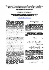
Fig. 3: Domain of the experiment. A 2.2 × 2.2 × 0.4m3 box with velocity inlet at bottom right and outlet at bottom left. The origin of the coordinate system is located at bottom left corner.

u(x), v(x), and the turbulent intensity i(x) are independent, their joint likelihood is the multiplication of their individual likelihoods. Given these likelihoods, the posterior discrete probability of the models given the current measurements is obtained from (22). Finally, given the model probabilities and the posterior turbulent intensity field, in line 12, the planning problem (42) is solved using Algorithm 2 to determine the next measurement location. As the number of collected measurements increases, the amount of information added by a new measurement will decrease since the entropy is a submodular function. This means that the posterior estimates of the mean velocity field and turbulent intensity will converge. Thus to terminate Algorithm 3, in line 10 we check the change in these posterior fields averaged over the model probabilities. Particularly, we check if n ¯ X dk = pj,k (du,k,j + dv,k,j + di,k,j ) < tol, (44) j=1

where tol is a user-defined tolerance and the difference in posterior fields of u(x) at iteration k, is given by Z 1 ˆ du,k,j = |µu (x | Xk , Mj ) − µu (x | Xk−1 , Mj )| d Ω, ˆ |Ω| (45) ˆ is the area of the projected 2D domain. The other where |Ω| two values dv,k,j and di,k,j are defined in the same way. V. E XPERIMENTAL R ESULTS In this section we present experimental results to demonstrate the performance of Algorithm 3. Particularly, we consider a 2.2 × 2.2 × 0.4m3 domain with an inlet, an outlet, and an obstacle inside as shown in Figure 3. We assume that the

12

A. Signal Processing In order to examine the accuracy of the probabilistic measurement models developed in Section III-B, we conduct a series of experiments where we collect 25 measurements of the flow properties at two locations x1 = (1.9, 0.4) and x2 = (0.35, 0.4). x1 is located at a high velocity region whereas x2 is located at a low velocity region. The instantaneous samples of u(x1 ) and v(x1 ) are given in Figure 4 for the first measurement. A video of the instantaneous velocity readings can be found in [49]; note the amount of fluctuations in the

1 0.8 0.6 0.4

velocity (m/s)

origin of the coordinate system is located at the bottom left corner of the domain. We use a fan to generate a flow at the inlet with average velocity qin = 0.78m/s. As discussed in Section IV-A, we construct a custom mobile sensor to carry out the experiment. To minimize the interference with the flow pattern and since the domain is small, we use a small differential-drive robot to carry the flow sensors and collect the measurements. We equip the mobile robot with an A RDUINO L EONARDO microprocessor that implements simple motion primitives and collects instantaneous velocity readings and communicates them back to an off-board PC for processing. The radio communications between the mobile sensor and the PC happen via a network of X BEE -S2s. The PC processes the instantaneous readings, the localization information, and runs Algorithm 3 using MATLAB. As discussed in Section IV-A, the mobile sensor is also equipped with eight D6F-W01A1 OMRON sensors with range of 0 − 1m/s and full-scale error rate of FS = 0.05m/s. We set the standard deviation of the sensor noise to γs = 0.017m/s according to (27), the heading error to γβ = 5o , and the measurement location error to γx = 0.025m. We construct a SROM model for the location error with n ˜ = 5 samples; see Section IV-B. Note that the location error also takes into account the discretization of the numerical solutions and the error caused by the sensor rig structure. In order to control the mobile sensor between consecutive waypoints to collect the measurements, we decouple its motion into heading control and straight-line tracking. The low level planning to generate these straight-line trajectories while avoiding the obstacles can be done in a variety of ways; here we use geodesic paths proposed in [48]. The feedback required for motion control is provided by an O PTI T RACK motion capture system. The robot stops when the distance between the desired and final locations is below a threshold. A similar condition is used for the heading angle. In the following, we first discuss how to process the instantaneous velocity readings and demonstrate the accuracy of the probabilistic measurement models developed in Section III-B. Then, we show that Algorithm 3 (i) correctly selects models that are in agreement with empirical data, (ii) converges as the number of measurements m increases and, most importantly, (iii) predicts the flow properties more accurately than the prior numerical models while providing reasonable uncertainty bounds for the predictions. Finally, we also demonstrate that the entropy information metric for planning outperforms other metric, such as the mutual information.

0.2 0 -0.2 -0.4 -0.6 u(x,t)

v(x,t)

u(x)

v(x)

-0.8 0

5

10

15

20

25

30

time (s)

Fig. 4: The instantaneous velocity components at x1 for first measurement where u(x) = −0.07m/s and v(x) = 0.63m/s.

Fig. 5: Histogram of 25 independent measurements of u(x1 ).

velocity vector. The robot samples the velocity vector with a fixed frequency of 67Hz. Then, to ensure that the samples are uncorrelated, it down-samples them using the integral time scale; see Section III-C3. The average integral time scales over 25 measurements are t¯∗ (x1 ) = 0.26s and t¯∗ (x2 ) = 0.29s, respectively. Figure 5 shows a histogram of the 25 independent u(x1 ) measurements. This histogram approaches a Gaussian distribution as the number of measurements increases. Histograms of the second component and turbulent intensity are similar for both points. Next, Figure 6 shows the measurements of the velocity vector at x1 . In Figure 7, we plot the sample standard deviations of the velocity components and turbulent intensity, obtained from equations (15) and (21), for both locations. Note that for the velocity components, the average standard deviation values are close indicating that the isotropy assumption is appropriate. In Table I, we compare the standard deviations obtained from each measurement, averaged over all experiments, to the standard deviation of measurements from all 25 experiments. We refer to the former as withinexperiment and the latter as cross-experiment. Note that the cross-experiment values, reported in the second column, are

13

velocity at x1

0.04

1.1

sd of u(x 1 ) sd of v(x 1 )

1

0.035

mean sd of u(x 1 ) mean sd of v(x1 )

0.9

0.8 measurements mean

0.7

velocity (m/s)

0.03

0.025

0.02 0.6 0.015

0.5

0.4

0.01 1.5

1.6

1.7

1.8

1.9

2

2.1

2.2

2.3

0

5

10

15

20

25

measurement number

(a) standard deviations of velocity components for x1

Fig. 6: 25 measurements of the velocity vector at x1 = (1.9, 0.4) along with their averaged vector.

0.018 sd of u(x 2 )

TABLE I: Standard deviation values. within-exp

mean sd of u(x 2 ) mean sd of v(x2 )

cross-exp 0.014

u(x1 )

sd of sd of v(x1 )

0.024 0.021

0.120 0.042

sd of u(x2 ) sd of v(x2 )

0.012 0.011

0.038 0.023

sd of i(x1 ) sd of i(x2 )

0.014 0.010

0.026 0.015

velocity (m/s)

method

sd of v(x 2 )

0.016

0.012

0.01

0.008

0.006

larger. This is due to actuation errors that are not considered within experiments but appear across different measurements, i.e., the experiments corresponding to location x1 for instance, are not all conducted at the same exact location and heading of the robot. The small number of experiments may also contribute to inaccurate estimation of the standard deviations in the second column.

0.004 0

5

10

15

20

25

measurement number

(b) standard deviations of velocity components for x2 0.02 0.018

B. Inference In this section, we illustrate the ability of Algorithm 3 to select the best numerical model and to obtain the posterior distribution of the flow properties. Particularly, we utilize ANSYS F LUENT to solve the RANS models for the desired flow properties using the k − , k − ω, and RSM solvers. We assume uncertainty in the inlet velocity and turbulent intensity values. This results in n ¯ = 12 different combinations of BCs and RANS models; see the first four columns in Table II for details. In the third column, ‘profile’ refers to cases where the inlet velocity is modeled by an interpolated function instead of the constant value qin = 0.78m/s. Columns 5 and 6 show the prior uncertainty in the solutions of the first velocity component and turbulent intensity; cf. equation (4). We set σ ¯v = σ ¯u . As discussed in Section III-B, these values should be selected to reflect the uncertainty in the numerical solutions. Here, we use the residual values from ANSYS F LUENT as an indicator of the confidence in each numerical solution. Figure 8 shows the velocity magnitude fields obtained using models 1 and 2. The former is obtained using the k −  model whereas the latter is obtained using the RSM, as reported

turbulent intensity (%)

0.016 0.014 0.012 0.01 0.008

sd of i(x 1 ) sd of i(x 2 ) mean sd of i(x 1 )

0.006

mean sd of i(x 2 )

0.004 0

5

10

15

20

25

measurement number

(c) standard deviations of turbulent intensity

Fig. 7: Standard deviations of velocity components and turbulent intensity obtained for each of 25 measurement in both locations x1 = (1.9, 0.4) and x2 = (0.35, 0.4).

in Table II. Note that these two solutions are inconsistent and require experimental validation to determine the correct flow pattern. We initialize Algorithm 3 by assigning uniform probabilities to all models in Table II, i.e., pj,0 = 1/¯ n for

14

TABLE II: Numerical solvers and uncertain parameters. No.

model

qin (m/s)

iin (%)

σ ¯u (m/s)

σ ¯i (%)

1 2 3 4 5 6 7 8 9 10 11 12

k− RSM k−ω k− RSM k−ω RSM RSM RSM RSM RSM RSM

0.78 0.78 0.78 profile profile profile profile profile profile profile 0.76 0.80

0.02 0.02 0.02 0.02 0.02 0.02 0.05 0.03 0.01 0.04 0.03 0.03

0.10 0.20 0.20 0.14 0.20 0.20 0.14 0.20 0.20 0.20 0.20 0.14

0.05 0.10 0.10 0.07 0.10 0.10 0.07 0.10 0.10 0.10 0.10 0.07

Fig. 9: Path of the mobile sensor according to the entropy metric overlaid on the turbulent intensity field from model 7. The green dots show the candidate measurement locations and the yellow stars show the exploration measurement locations. Finally, the black dots show the sequence of waypoints.

(a) numerical solution using k −  model

(b) numerical solution using RSM

Fig. 8: Predictions of the velocity magnitude field (m/s) according to models 1 and 2 in the plane of the mobile sensor located at the height of 0.27cm.

1≤j ≤n ¯ . We use m ¯ = 16 exploration measurements and set the maximum number of measurements to m = 200. The

convergence tolerance in (44) is set to tol = 10−4 m/s. Figure 9 shows the sequence of waypoints generated by Algorithm 2. For these results, we use a correlation characteristic length of ` = 0.35m. This value provides a reasonable correlation between each measurement and its surroundings and guarantees an acceptable spacing between waypoints. The green dots in Figure 9 show the 1206 candidate measurement locations, collected in the set S, and the yellow stars show the m ¯ = 16 exploration measurement locations selected over a lattice. The black dots show the sequence of waypoints returned by Algorithm 2. Note that as the size of the set S grows, it will take longer to evaluate all candidate locations in Algorithm 2. The resolution of these candidate locations should be selected in connection with the characteristic length `. For the larger values of `, the resolution could be lower. Note also that the computations of the entropy metric (43) at different locations are independent and can be done in parallel. Finally, for very large domains we can consider a subset of candidate measurement locations from the set S that lie in the neighborhood of the current location of the robot at every step. Algorithm 3 converges after k = 164 measurements. Figure 10 shows the amount of added information using the entropy metric (43) after the addition of each of these measurement. It can be observed that the amount of added information generally decreases as the mobile sensor keeps adding more measurements. This is expected by the submodularity of the entropy information metric. Figure 11 shows the collected velocity vector measurements. Referring to Figure 8, observe that this vector field qualitatively agrees with model 2 that was obtained using the RSM. Also, Figure 12 shows the evolution of the convergence criterion (44) of Algorithm 3. The high value of this criterion for measurement m ¯ = 16 corresponds to conditioning on all exploration measurements at once; the

15

10-1

0.02

raw data smoothed data

0.019

convergence criterion (m/s)

added information (m/s)2

0.018 0.017 0.016 0.015 0.014 0.013

10-2

10-3

0.012 0.011 20

40

60

80

100

120

140

160

measurement number

10-4 20

Fig. 10: Added information δIH (x) as a function of measurement number for entropy metric.

40

60

80

100

120

140

160

measurement number

Fig. 12: Evolution of convergence criterion (44) as a function of measurement number k. (24), are given. Comparing the prior and posterior velocity fields, we observe a general increase in velocity magnitude at the top-left part of the domain indicating that the flow sweeps the whole domain unlike the prior prediction from model 7; see also Figure 11. Furthermore, comparing the prior and posterior turbulent intensity fields, we observe a considerable increase in turbulent intensity throughout the domain. Referring to Table II, note that among all RSM models, model 7 has the highest turbulent intensity BC. In [50], a visualization of the flow field is shown that validates the flow pattern depicted in Figures 11 and 13.

2

1.5

1

0.5

C. Prediction

0 0

0.5

1

1.5

2

Fig. 11: Velocity vector measurements for entropy metric.

next measurements do not alter the posterior fields as much. The posterior probabilities pj,k converge once the exploration measurements are collected, i.e., at iteration k = m, ¯ and do not change afterwards. Particularly, the numerical solution from the RSM model 7 is the only solution to have nonzero probability, i.e., p7,164 = 1.00. This means that the most accurate model can be selected given a handful of measurements that determine the general flow pattern. It is important to note that all solutions provided by RSM share a similar pattern and the empirical data help to select the most accurate model. Note also that these posterior probabilities are computed given ‘only’ the available models listed in Table II. Thus, they should only be interpreted with respect to these models and not as absolute probability values. In Figure 13, the prior velocity magnitude and turbulent intensity fields corresponding to the most probable model, i.e., model 7, and the posterior fields, computed using equations

Next, we compare the accuracy of the posterior fields against the pure numerical solutions given by the RANS models. To this end, we randomly select a set of m ˆ new locations and collect measurements at these locations. Let yˆu (xl ) denote the measurement of the first velocity component at a location xl for 1 ≤ l ≤ m. ˆ Let also µu (xl |Xk ) denote the predicted mean velocity obtained from (24a) after conditioning on the previously collected measurements Xk up to iteration k of Algorithm 3. Then, we define the mean error over the random locations xl as m ˆ

eu,k =

1 X |µu (xl |Xk ) − yˆu (xl )| , m ˆ

(46)

l=1

and finally ek = 1/3(eu,k +ev,k +ei,k ), where the expressions for ev,k and ei,k are identical. We are particularly interested in e0 as the prediction error of the numerical solutions and em as the prediction error of the posterior field. For a set of m ˆ = 20 randomly selected test locations, we obtain e0 = 0.090m/s and an average posterior error e164 = 0.037m/s which is 59% smaller than e0 . Given the posterior knowledge that model 7 has the highest probability, we also compute e¯0 where we use µu (xl |Xk , M7 ) in definition (46) instead of the mean value from (24a). We do the same for v(x) and i(x). In this case, the error using the prior numerical model is e¯0 = 0.060m/s

16

(a) prior velocity magnitude field (m/s) from model 7

(b) prior turbulent intensity field from model 7

(c) posterior velocity magnitude field (m/s)

(d) posterior turbulent intensity field

Fig. 13: The prior fields from model 7 and the posterior fields obtained using equations (24) after conditioning on empirical data.

which is still 38% higher than the posterior error value e164 . This demonstrates that the real flow field can be best predicted by systematically incorporating the theoretical models and empirical data. Note that this hypothetical scenario requires the knowledge of the best model which is not available a priori. In Figure 14, we plot the prior errors for all models together with the posterior errors for u, v, and i, separately. It can be seen that the solutions using the RSM models, including model 7, have smaller errors; see also Table II. As discussed at the beginning of this section, an important advantage of the proposed approach is that it provides uncertainty bounds on the predictions. Figure 15 shows the values of the individual measurements at each one of the m ˆ measurement locations along with the posterior predictions and their uncertainty bounds. We also include error bars for the measurements that fall outside these uncertainty bounds. In Figure 15a, four measurements of the first velocity component

fall outside the one standard deviation bound. Similarly, three and one measurements of the second velocity component and the turbulent intensity are outside this bound; see Figures 15b and 15c. This shows that the proposed method provides uncertainty bounds that are neither wrong nor conservative. D. Planning Optimality Finally, we show that the proposed planning method using the entropy metric outperforms other similar metrics, such as the Mutual Information (MI) metric which has a suboptimality lower-bound. Using the same notation introduced in Section IV-C, let I(X , Ω\X ) denote the MI between measurements X and unobserved regions of the domain Ω\X , given by I(X , Ω\X ) = H(Ω\X ) − H(Ω\X | X ). Denote this value by I(X ) for short. Then, the amount of added information by a new measurement x ∈ S\X is

17

0.3

0.25

prediction observation

u (m/s) v (m/s) i (%)

0.2

0.2

0.15

u (m/s)

average error value

0.1

0

-0.1

0.1 -0.2

0.05

-0.3

-0.4 0

8

10

12

14

16

18

20

r

st e

rio

r

6

(a) first velocity component 0.8 prediction observation

0.6

0.4

v (m/s)

δIMI (x | X ) = I(X ∪x)−I(X ) = H(x | X )−H(x | X¯ ), where X¯ = Ω\(X ∪x); see [31] for details of derivation. Particularly, for a GP using the definiton of the entropy in (41) we get

0.2

0

(47)

[31] show that under certain assumptions on the discretization Ω, MI is a monotone and submodular set function. Then, according to the maximization theory of submodular functions, the suboptimality of Algorithm 2 is lower-bounded when δIMI is used; see [30]. In order for this suboptimality bound to hold, we do not update the model probabilities pj,k in (42). To compare the two metrics, we use similar settings as those in Section V-B and set the maximum number of measurements to m = 30. Figure 16 shows the sequence of waypoints generated by Algorithm 2 for the entropy and MI metrics, respectively. It is evident that the entropy metric signifies regions with higher variations of velocity field whereas the MI metric is more sensitive to correlation; see also equations (43) and (47). Conditioning on the measurements collected using these metrics, the prediction errors for the same m ˆ = 20 test locations, are e30 = 0.042 for the entropy metric and e30 = 0.047 for the MI metric, respectively. Thus, the entropy metric outperforms the MI metric by 11%. Note that with only m = 30 measurements, the error in the posterior fields is considerably smaller than the prior value e0 = 0.090. Nevertheless, convergence requires more measurements as we demonstrated in Section V-B. Note also that depending on the size of the discrete domain Ω, the covariance matrix ΣX¯ X¯ can be very large. This makes the evaluation of the MI metric (47) considerably more expensive than the entropy metric. VI. C ONCLUSION In this paper we proposed a model-based learning method that relies on mobile robot sensors to improve on the numerical solutions of turbulent flow fields obtained from RANS models.

-0.2

-0.4 0

2

4

6

8

10

12

14

16

18

20

measurement number

(b) second velocity component 0.25 prediction observation

0.2

turbulent intensity (%)

γu2 (x | X ) . γu2 (x | X¯ )

4

measurement number

Fig. 14: Prior error values for individual models along with their averaged prior as well as the posterior errors eu,164 , ev,164 , and ei,164 .

δIMI (x | X ) ∝

2

po

12

io pr

11

el

el

od

od

m

9

10 el

od

m

8

el od

m

m

7 od

el

6

el od

m

m

5 od

el

4

el od

m

m

3 od

el

2

el od

m

m

el od

m

m

od

el

1

0

0.15

0.1

0.05

0

-0.05 0

2

4

6

8

10

12

14

16

18

20

measurement number

(c) turbulent intensity

Fig. 15: Posterior predictions and their uncertainty bounds at m ˆ test locations along with the measured values shown by red stars. We also plot the error bounds on the measurements that fall outside the uncertainty bounds.

Particularly, we constructed a statistical model of the flow using Gaussian Processes (GPs) whose mean was informed by the numerical solutions obtained from RANS models. We then utilized Bayesian inference to incorporate empirical

18

ACKNOWLEDGEMENTS The authors would like to thank Dr. Wilkins Aquino for providing access to ANSYS F LUENT, Dr. Scovazzi for his valuable inputs on turbulence, and Eric Stach and Yihui Feng for their help in designing the experimental setup and the mobile sensor. R EFERENCES

(a) entropy metric

(b) mutual information metric

Fig. 16: Path of the mobile sensor for two optimality metrics overlaid on turbulent intensity field from model 7. The green dots show the candidate measurement locations and the yellow stars show the exploration measurement locations. Finally, the black stars show the sequence of waypoints.

measurements of the flow field into these GPs. To the best of our knowledge, our method is the first model-based framework that can be used to learn flow fields using empirical data. We designed a cost-effective flow sensor mounted on a custombuilt mobile robot that collects and analyzes instantaneous velocity readings. We presented experimental results demonstrating that the proposed framework can select the most accurate models, obtain the posterior distribution of the flow properties and, most importantly, predict these properties at new locations with reasonable uncertainty bounds. Our results showed considerable improvement in the prediction of the flow field properties compared to pure numerical simulations.

[1] G. A. Hollinger, A. A. Pereira, J. Binney, T. Somers, and G. S. Sukhatme, “Learning uncertainty in ocean current predictions for safe and reliable navigation of underwater vehicles,” Journal of Field Robotics, vol. 33, no. 1, pp. 47–66, 2016. [2] K.-C. Ma, L. Liu, and G. S. Sukhatme, “An information-driven and disturbance-aware planning method for long-term ocean monitoring,” in Proceedings of IEEE International Conference on Intelligent Robots and Systems, pp. 2102–2108, IEEE, 2016. [3] S. A. Thorpe, An introduction to ocean turbulence. Cambridge University Press, 2007. [4] R. B. Stull, An introduction to boundary layer meteorology, vol. 13. Springer Science & Business Media, 2012. [5] J. Lee, H. Ghorbanidehno, M. W. Farthing, T. J. Hesser, E. F. Darve, and P. K. Kitanidis, “Riverine bathymetry imaging with indirect observations,” Water Resources Research, vol. 54, no. 5, pp. 3704–3727, 2018. [6] S. Pang and J. A. Farrell, “Chemical plume source localization,” IEEE Transactions on Systems, Man, and Cybernetics, Part B, vol. 36, no. 5, pp. 1068–1080, 2006. [7] H. B. Awbi, Ventilation of buildings. Routledge, 2002. [8] J. S. Parsons, R. E. Goodson, and F. R. Goldschmied, “Shaping of axisymmetric bodies for minimum drag in incompressible flow,” Journal of Hydronautics, vol. 8, no. 3, pp. 100–107, 1974. [9] P. Dyverfeldt, R. G˚ardhagen, A. Sigfridsson, M. Karlsson, and T. Ebbers, “On MRI turbulence quantification,” Magnetic Resonance Imaging, vol. 27, no. 7, pp. 913–922, 2009. [10] M. Forghani, W. Huang, and M. K. Jawed, “Control of uniflagellar soft robots at low Reynolds number using buckling instability,” 2018. . ArXiv: https://arxiv.org/abs/1810.03113. [11] R. Khodayi-mehr, W. Aquino, and M. M. Zavlanos, “Model-based sparse source identification,” in Proceedings of American Control Conference, pp. 1818–1823, July 2015. [12] R. Khodayi-mehr, W. Aquino, and M. M. Zavlanos, “Nonlinear reduced order source identification,” in Proceedings of American Control Conference, pp. 6302–6307, July 2016. [13] R. Khodayi-mehr, W. Aquino, and M. M. Zavlanos, “Modelbased active source identification in complex environments,” IEEE Transactions on Robotics, 2018. (accepted). [Online]. Available: https://arxiv.org/pdf/1706.01603.pdf. [14] G. K. Batchelor, An introduction to fluid dynamics. Cambridge university press, 2000. [15] D. C. Wilcox, Turbulence modeling for CFD, vol. 2. DCW Industries La Canada, CA, 1993. [16] P. Hanafizadeh, M. Momenifar, A. N. Geimassi, and S. Ghanbarzadeh, “Void fraction and wake analysis of a gas-liquid two-phase cross-flow,” Multiphase Science and Technology, vol. 26, no. 4, 2014. [17] J. Ling and J. Templeton, “Evaluation of Machine Learning algorithms for prediction of regions of high Reynolds averaged navier stokes uncertainty,” Physics of Fluids, vol. 27, no. 8, p. 085103, 2015. [18] F. E. Jorgensen, How to measure turbulence with hot-wire anemometers: a practical guide. Dantec dynamics, 2001. [19] M. Raffel, C. E. Willert, J. Kompenhans, et al., Particle image velocimetry: a practical guide. Springer Science & Business Media, 2007. [20] F. Durst, A. Melling, and J. H. Whitelaw, “Principles and practice of laser-doppler anemometry,” NASA STI/Recon Technical Report A, vol. 76, 1976. [21] L. L¨ofdahl and M. Gad-el Hak, “Mems applications in turbulence and flow control,” Progress in Aerospace Sciences, vol. 35, no. 2, pp. 101– 203, 1999. [22] S. M¨uller, M. Milano, and P. Koumoutsakos, “Application of Machine Learning algorithms to flow modeling and optimization,” Center for Turbulence Research Annual Research Briefs, Stanford University, pp. 169– 178, 1999. [23] J. Tompson, K. Schlachter, P. Sprechmann, and K. Perlin, “Accelerating Eulerian fluid simulation with convolutional networks,” arXiv preprint arXiv:1607.03597, 2016.

19

[24] S. Jeong, B. Solenthaler, M. Pollefeys, M. Gross, et al., “Data-driven fluid simulations using regression forests,” ACM Transactions on Graphics, vol. 34, no. 6, p. 199, 2015. [25] I. Bright, G. Lin, and J. N. Kutz, “Compressive sensing based Machine Learning strategy for characterizing the flow around a cylinder with limited pressure measurements,” Physics of Fluids, vol. 25, no. 12, p. 127102, 2013. [26] Z. J. Zhang and K. Duraisamy, “Machine Learning methods for datadriven turbulence modeling,” in 22nd AIAA Computational Fluid Dynamics Conference, p. 2460, 2015. [27] I. Derevich and L. Zaichik, “An equation for the probability density, velocity, and temperature of particles in a turbulent flow modelled by a random Gaussian field,” Journal of Applied Mathematics and Mechanics, vol. 54, no. 5, pp. 631–637, 1990. [28] A. Tsinober, An informal introduction to turbulence, vol. 63. Springer Science & Business Media, 2001. [29] L. Benedict and R. Gould, “Towards better uncertainty estimates for turbulence statistics,” Experiments in Fluids, vol. 22, no. 2, pp. 129– 136, 1996. [30] G. L. Nemhauser, L. A. Wolsey, and M. L. Fisher, “An analysis of approximations for maximizing submodular set functions—i,” Mathematical Programming, vol. 14, no. 1, pp. 265–294, 1978. [31] A. Krause, A. Singh, and C. Guestrin, “Near-optimal sensor placements in Gaussian processes: Theory, efficient algorithms and empirical studies,” Machine Learning Research, vol. 9, pp. 235–284, 2008. [32] J. Le Ny and G. J. Pappas, “On trajectory optimization for active sensing in Gaussian process models,” in Proceedings of IEEE Conference on Decision and Control, pp. 6286–6292, IEEE, 2009. [33] F. Berkenkamp, R. Moriconi, A. P. Schoellig, and A. Krause, “Safe learning of regions of attraction for uncertain, nonlinear systems with gaussian processes,” in Proceedings of IEEE Conference on Decision and Control, pp. 4661–4666, IEEE, 2016. [34] F. Berkenkamp and A. P. Schoellig, “Safe and robust learning control with Gaussian processes,” in European Control Conference, pp. 2496– 2501, IEEE, 2015. [35] C. J. Ostafew, A. P. Schoellig, and T. D. Barfoot, “Learning-based nonlinear model predictive control to improve vision-based mobile robot path-tracking in challenging outdoor environments,” in Proceedings of IEEE International Conference on Robotics and Automation, pp. 4029– 4036, IEEE, 2014. [36] H. Wei, W. Lu, P. Zhu, S. Ferrari, R. H. Klein, S. Omidshafiei, and J. P. How, “Camera control for learning nonlinear target dynamics via Bayesian nonparametric Dirichlet-process Gaussian-process (DP-GP) models,” in Proceedings of IEEE International Conference on Intelligent Robots and Systems, pp. 95–102, IEEE, 2014.

[37] X. Lan and M. Schwager, “Learning a dynamical system model for a spatiotemporal field using a mobile sensing robot,” in Proceedings of American Control Conference, pp. 170–175, IEEE, 2017. [38] X. Lan and M. Schwager, “Planning periodic persistent monitoring trajectories for sensing robots in Gaussian random fields,” in Proceedings of IEEE International Conference on Robotics and Automation, pp. 2415– 2420, IEEE, 2013. [39] C. Freundlich, S. Lee, and M. M. Zavlanos, “Distributed active state estimation with user-specified accuracy,” IEEE Transactions on Automatic Control, June 2017. [40] C. Freundlich, P. Mordohai, and M. M. Zavlanos, “Optimal path planning and resource allocation for active target localization,” in Proceedings of American Control Conference, pp. 3088–3093, IEEE, 2015. [41] R. Khodayi-mehr, Y. Kantaros, and M. M. Zavlanos, “Distributed state estimation using intermittently connected robot networks,” IEEE Transactions on Robotics, 2018. (accepted). [Online]. Available: https://arxiv.org/pdf/1805.01574.pdf. [42] C. E. Rasmussen and C. K. Williams, Gaussian processes for Machine Learning, vol. 1. Cambridge: MIT press, 2006. [43] K. Wolter, Introduction to variance estimation. Springer Science & Business Media, 2007. [44] H. Hassani, “Sum of the sample autocorrelation function,” vol. 17, pp. 125–130, 08 2009. [45] P. L. O’Neill, D. Nicolaides, D. Honnery, and J. Soria, “Autocorrelation functions and the determination of integral length with reference to experimental and numerical data,” 01 2004. [46] L. Calkins, R. Khodayi-mehr, W. Aquino, and M. Zavlanos, “Stochastic model-based source identification,” in Proceedings of IEEE Conference on Decision and Control, pp. 1272–1277, 2017. [47] M. F. Huber, T. Bailey, H. Durrant-Whyte, and U. D. Hanebeck, “On entropy approximation for Gaussian mixture random vectors,” in Multisensor Fusion and Integration for Intelligent Systems, pp. 181–188, IEEE, 2008. [48] K. J. Obermeyer and Contributors, “The VisiLibity library.” http://www.VisiLibity.org, 2008. Release 1. [49] R. Khodayi-mehr and M. M. Zavlanos, “Instantaneous velocity vector https://vimeo.com/281186744,” 2018. [50] R. Khodayi-mehr and M. M. Zavlanos, “Flow visualization - https:// vimeo.com/281498120,” 2018.