that indicate the spam category in the email collections, such as cash and sex of Email1431, advertisement and unsolicit for LingSpam, and play and hot for ...
〚䇻㚄㾮⭥㵗䇑㈼㏁Ⳟⳉ
᎖ෝቯࡼᄾ፬ಢऱज Model-Based Method for Projective Clustering* Lifei Chen, Qingshan Jiang and Shengrui Wang ᐢ! ገ! 㬽㸍Ⱙ㾈䇇䇑㼍᷍ⷀ㸍㭞㈾㈼㏁⧪㸋䄜䐹䄋⭥㳕䍞᱄㸋ㆃ㉗䎃㸫㳃᷍䄲㳂⨗㵗䇑㈼㏁Ⳟⳉ᷍䔘㸋⪌㵔㈼㏁⭥ 䄜䐷㎊䍚䊻㭞㈾㋶ヅ⭥㸍Ⱙ䓴ゐ䐱㯲㰘㵗䇑⪹㏁᱄⡟㸥㬸㻩㳂⨗䄜㘉㭗ⷀ㸍㋶ヅ㵗䇑⪹㏁⭥ⶦ㔫㵔ェ㚄㾮ᷜㅴ䓦᷍ⷙ⨗ 䄜〚䇻㚄㾮⭥㚄⽞㵗䇑㈼㏁㰄ⳉ᷍䇤䇻䊻⤜㵍⭥㵗䇑㋶ヅ䐱ⳃ㻷⢀ㆈ䐹⮟⭥⪹㏁᱄㾣Ⳟⳉ䊻⼰⧪㭞㈾⼮䄜㾊⧄䇤⭥㬖カ 㭞㈾ゐ㩰㆙㾱㑬㬖䂊䂊䐅᱄ ਈࠤ! ㈼㏁ᷜⷀ㸍ᷜ㵗䇑㈼㏁ᷜⶦ㔫㚄㾮 ABSTRACT Clustering high-dimensional data is a major challenge due to the curse of dimensionality. To solve this ������� ����� ��� ��� ����� ��� ���� ������ �� �� �� ������
�
���� ����� ��� �����
�� �
��� �
� ��� ����� ��
��� ��� �� ����� � ��
�� ���������� �� � �� � ��� �� ��
��� ����� � ��������� � ����� �� ��� ��������
� ��� ����
projected clusters in high-dimensional data space. Then, we present a model-based algorithm for fuzzy projective clustering that discovers clusters with overlapping boundaries in various projected subspaces. The suitability of the proposal is demonstrated in an empirical study done with synthetic datasets and some widely used real-world datasets. KEYWORDS
���� ����� ���� ���������� !���� ��� ���� ����� !�������� � "����
1 Introduction spaces[7][8], making the Gaussian function inappropriate in this case. Verleysen[7] states that when the dimension increases, the percentage of the samples of a normalized multivariate Gaussian distribution falling around its center would rapidly decrease to 0. In other words, most of the volume of a Gaussian function is contained in the tails instead of near the center in high-dimensional space: the so-called “empty space phenomenon”[7].
D
ata clustering has a wide range of applications and has been studied extensively in the statistics, data mining and database communities. Many algorithms have been proposed in the area of clustering[1][2]. One popular group of such algorithms, the model-based methods, have sparked wide interest because of their additional advantages, which give them the capacity to describe the underlying structures of populations in the data[3].
Furthermore, in high-dimensional space, clusters may exist in different subspaces comprised of different combinations of features. In many real-world applications, in fact, some points are correlated with a given set of dimensions, and others are correlated with different dimensions. For example, in document clustering, clusters of documents on different topics are characterized by different subsets of keywords. The keywords for one cluster may not occur in the documents of other clusters. To address the above challenges, ������� ��� ���� ��������������������������� ������ �� different subspaces of the same dataset [9][10][11][29].
In model-based methods, data are thought of as originating from various possible sources, which are typically modeled by Gaussian mixture[3][4][5]. The goal is to identify the generating mixture of Gaussians, that is, the nature of each Gaussian source, with its mean and covariance. Examples include the classical k-means[1] [2] and its variants. However, such methods would suffer from the curse of dimensionality problem for highdimensional data[6]. Many types of real-world data, such as the documents represented in the Vector Space Model (VSM) used in text mining and the micro-array gene expression data of bioinformatics, consist of very high-dimensional features. The data are inherently sparse in high-dimensional
A projected cluster is an ensemble of subsets of points,
A��
C�
A��
A��
C�
A��
* A previous version of the paper appeared in IEEE Eighth International Conference on Data Mining (ICDM'08)[33]
A��
#��� /������ '��� �� ��������� �� �444 5����� ���� ��
Konowledge and Data Engineering,2012
A�
A�
#���$� % �� �� �� � ���� � �� &� ��� � ���
��
'�
projected clusters in 2D subspaces.
17
�
Vol. 5 No.11/ Nov. 2011 algorithm MPC. Experimental results are presented in Section 5. Finally, Section 6 gives our conclusion and discusses directions for future work.
each of which is associated with a subset of attributes. In Fig.1, two different projected clusters are illustrated for a set of data points in 3-dimensional space. There are two clusters in this example; however, they are associated � �������� �������� ���� ���� ��� �� ������������������ cluster corresponds to the data in group C1, which are close to each other when projected into the subspace consisting of the dimensions A1 and A2, while the second one corresponds to the data in group C2 projected onto the A1- A3 plane.
2 Related Work 2.1 Techniques for High-Dimensional Data Clustering Techniques for dimensionality reduction have been used in high-dimensional data clustering. Feature transformation techniques, such as PCA and SVD, attempt to summarize the dataset in a smaller number of new dimensions created via linear combination of the original attributes, while feature selection methods select only the most relevant attributes for the clustering task[10]. Because these traditional techniques are performed in the ��� ���������������������������� ������ ��� � �������� clusters are found in different subspaces. LDR(Local Dimensionality Reduction)[18] attempts to create a new set of dimensions for each cluster. The difficulties with a such method include the determination of dimensionality for each subspace associated with the clusters. Additionally, LDR often has high computational complexity.
A number of algorithms for finding such projected clusters have been proposed in the literature. They fall into two categories[12]�������� ����������������������� ��� include PROCLUS[9], ORCLUS[13] and FINDIT[14], are aimed at discovering the exact subspaces of different clusters. The algorithms in the second category cluster data points in the entire data space but assign different weighting values to different dimensions of clusters: examples include EWKM [12], FWKM [15] and LAC [16], most of the algorithms in the second category are of the k-means type, whose sequential structure is analogous to the mathematics of the EM algorithm[17]. However, there is a general lack of underlying models on which these methods can be built. In this paper, we will present a new model-based method for projective clustering. The first contribution is the proposal of a probability model to describe projected clusters in a high-dimensional space. In contrast to existing models for high-dimensional data clustering, our extended Gaussian model is designed for projective clustering, and by analysis is able to explain the general assumptions used in popular projective methods. Second, we derive an objective function for projective clustering based on the probability model and propose an EM-type, parameter-free algorithm, named MPC1, for optimizing the objective function. The performance of MPC has been evaluated on synthetic datasets and some widely used real-world datasets, and the experimental results show its effectiveness. The method presented in this paper is very different from the one in our previous work [33]. Although the basic density function of the projected cluster is reused, the probability model for projected clusters has been changed. This results in a different algorithm which is no more dependent on any user-defined parameter for updating the dimension weights. The new algorithm has been much better motivated, analyzed and experimentally evaluated.
Biclustering[21] also referred to as coclustering, has been proposed for simultaneous clustering on the data points and dimensions of high-dimensional data. One of its typical applications is in the analysis of gene expression data, where the task is to find subgroups of genes and subgroups of conditions such that the genes exhibit highly correlated activities for every condition. Finally, two related terms occur in the literature: subspace clustering and projective clustering. According to Parsons et al. [10], projective clustering algorithms constitute a particular category of the subspace clustering techniques. However, different views are put forward elsewhere in the literature: see for instance [11][23][29]. We adopt the taxonomy of [23] and make a distinction between the two terms based on the ideas behind them. The idea of subspace clustering is to identify all dense regions in all subspaces, whereas in projective clustering the main focus is on discovering clusters that are projected onto particular spaces. In the subspace � ���� ����� �����!"#$[34] was the pioneering approach, followed by a number of algorithms such as ENCLUS[35] and MAFIA[36] and SUBCLU[37]. The major concern of this paper is projective clustering. In the following pages, we will focus only on such techniques.
The remainder of this paper is organized as follows. Section 2 presents some related work and the rationale for our work. In Section 3, the projective clustering model is presented. Section 4 describes the new 1
2.2 Projective Clustering Methods Projective clustering is typically based on feature weighting [10][11] . Each dimension of each cluster is
MPC stands for Model-based Projective Clustering.
18
〚䇻㚄㾮⭥㵗䇑㈼㏁Ⳟⳉ Instead of identifying hard subspaces for clusters, the algorithms in the second category assign weights in the range [0,1]. Since the weights can be any real number in [0,1], we can call these soft projective clustering algorithms. Typically, the weight value for a dimension in a cluster is inversely proportional to the dispersion of the values from the center in the dimension of the cluster. In other words, a high weight indicates a small dispersion in a dimension of the cluster. Virtually all of the existing algorithms in this category are based on the following general assumptions [23]: (1) the data project along a � �� ������� ���� ������������� ������������ � �������� on the other dimensions; (2) the data are more likely to be uniformly distributed along each irrelevant dimension. We will examine the capabilities of our projective clustering model, presented below, with respect to these two general assumptions.
assigned a weighting value, indicating to what extent the dimension is relevant to the cluster. Usually, the weighting values of a given dimension may be different for different clusters. Based on the way the weights are determined, projective clustering algorithms can be divided into two categories: hard subspace clustering and soft subspace clustering[12]. !�������������������������� ���� ����������� ������� ����� with values of either 0 or 1, resulting in hard feature weighting for the subspaces. PROCLUS [9] , which is based on the traditional k-medoids approach, is a representative algorithm using this weighting scheme. PROCLUS samples the data, then selects a set of medoids and iteratively improves the clustering, with the goal of minimizing the average within-cluster dispersion. For each medoid, a set of dimensions is chosen whose average distances to the medoid are small compared to statistical �%������ ����&���������� ���������� ������� ���� �������� average Manhattan segmental distance is used to assign points to medoids. PROCLUS requires users to provide the average number of relevant dimensions per cluster, which is usually unknown to users.
A number of soft projective clustering algorithms have been reported recently[12][15][16][22] [25][38]. In [22], an algorithm makes use of particle swarm optimization is presented. Since a heuristic global search strategy is used, the near-optimal feature weights could be obtained by this algorithm; however, it would run more slowly ������������ ��� ���������� ��������� ���������������� �� clustering algorithm, the k-means type structure has been widely adopted. Based on the classical k-means clustering process[1], an additional step for computing the weighting values is added in each iteration in these algorithms, which include EWKM[12], FWKM[15], LAC[16], and FSC[25] etc. Algorithm 1 shows a typical structure for these algorithms.
FINDIT[14], which uses a distance measure called the Dimension Oriented Distance (DOD), is similar in structure to PROCLUS. As a hierarchical clustering algorithm, HARP [26] automatically determines the relevant attributes of each cluster without requiring userdefined parameters. HARP is based on the assumption that two data points are likely to belong to the same cluster if they are very similar to each other along many dimensions. DOC [27] also defines the subspace as a subset of attributes on which the projection of points in a partition is contained within a segment. DOC computes projected clusters using a randomized algorithm to minimize a certain quality function. MINECLUS [28] improves on DOC by transforming the problem of ��� ������������������ ������ ������������ ������� � ��� the frequent itemset.
�
�
,QSXW��WKH�GDWDVHW�DQG�WKH�QXPEHU�RI�FOXVWHUV�.�� 2XWSXW��7KH�SDUWLWLRQV�&�DQG�DVVRFLDWHG�ZHLJKW�YHFWRUV�:�� � EHJLQ� � � )LQG�WKH�LQLWLDO�FOXVWHU�FHQWHUV�9�DQG�VHW�:�ZLWK�HTXDO�YDOXHV�� 5HSHDW� ���5H�JURXS�WKH�GDWDVHW�LQWR�&�DFFRUGLQJ�WR�WKH�9�DQG�:�� � ���5H�FRPSXWH�9�DFFRUGLQJ�WR�WKH�&�� ���5H�FRPSXWH�:�DFFRUGLQJ�WR�WKH�&�� � 8QWLO�FRQYHUJHQFH�LV�UHDFKHG�� HQG�
PROCLUS[9] and the other algorithms mentioned above search for axis-aligned subspaces for the clusters, while some other methods search more general subspaces, termed non-axis-aligned [24], where the new features are linear combinations of the original dimensions. ORCLUS[13] is a generalization of PROCLUS that can discover clusters in arbitrarily oriented subspaces. By covariance matrix diagonalization, ORCLUS selects the eigenvectors corresponding to the smallest eigenvalues of the matrix of the set of points. ORCLUS inherits the weaknesses of PROCLUS mentioned above. KSM[29], a k-means type projective clustering algorithm, determines the non-axis-aligned subspaces by SVD computations, while EPCH[30] performs non-axis-aligned projective clustering by histogram construction.
�
Algorithm1: A k-mean-type projective clustering algorithm. From Algorithm 1, the common projective clustering algorithm can be thought of as an EM-based process for estimating the unknown parameters C,V and W of a model F(C,V,W) from which the data originate. However, the underlying F(C,V,W) is generally neglected in the above methods. The lack of such a model makes derivation of more effective clustering algorithms � ��� �[20]. This has led us to work on projected cluster modeling, since we are convinced this type of modeling process allows us to benefit from the full potential of cluster analysis: for example, in describing the
19
Vol. 5 No.11/ Nov. 2011 underlying mechanism that generates the cluster structure and addressing cluster validity problems.
Table 1. Notation used throughout the paper
In a typical model-based clustering analysis, one tries to find a mixture of multivariate distributions to approximate the data. Due to the empty space phenomenon and the property of projective clustering, as mentioned above, cluster modeling on high-dimensional data is a difficult problem. In one of the few attempts to use model-based high-dimensional data clustering, Hoff[19] proposed a model of “clustering shifts in mean and variance” based on a nonparametric mixture of sequences of independent normal random variables. The model is learned by a Markov chain Monte Carlo process; however, its computational cost is prohibitive. Harpaz et al. [20] presented a non-parametric density estimation modeling technique, where the data are described as a mixture of linear manifolds. A Bayesian ��������� �� ������� ���� ������ �������� ��������������� are embedded in lower-dimensional linear manifolds. The low-dimensional subspaces associated with the individual clusters are computed by PCA. The problems with this method lie in its inflexibility in determining the dimensionality of the subspaces, and its inefficient clustering process.
.
(1)
The cluster c k is associated with a weight vector 3 , satisfying (2) Here the weight wk� ���������������� ��������� � ����� of the jth dimension to ck. The greater the relevance, the larger the weight. Furthermore, we introduce a D×D matrix sk���� ��� ������������
3 A Probability Model for Projective Clustering
T
he attributes of a non-axis-aligned subspace are typically combinations of the dimensions of the �� � �� �������������' �������������� ��� ����� ���������� often making the clustering results less useful for many real applications[10], such as document clustering, only projected clusters in axis-aligned subspaces are formalized in the following presentation.
For a given ck the assignment of can be regarded as a soft feature selection procedure for the space in which ck exists[16]. We thus use such a matrix to stand for the subspace associated with a cluster. The ���� � ����������������� ������ ��� ��� ��*��� � ���+�
������� �� � ���������� �� The notation used throughout the paper is summarized in Table 1. Given a dataset
be the ��������� �(Projected Cluster) Let kth projected cluster of DB, where denotes the membership degrees of all the data points with regard to the kth cluster, k=1,2,…,K.
c o n t a i ni ng K
clusters, for i=1,2,…,N are called data points in the D-dimensional space. It is assumed that the dataset has been normalized2 such that each where j=1,2,…,D. The membership degree of xi with regard to the kth cluster ck, where k=1,2,…,K, is denoted as uki, subject to the following constraints:
In order to examine the distribution of data points in a projected cluster, we need to project them onto their subspaces. ��������� (Projection) Let x be a data point of PCk and y its projection in its subspace,
2
In projective clustering, the dimension weight generally depends on the dispersion of the values in each dimension. So in order to obtain a meaningful set of weights, the values in all the dimensions need to be normalized into the same range. 3
;����� � ���'��� ��� ���� '� ���
��
��� �� ��
�
mean row vector.
(3) Let us examine the above definitions in the following derivation. Considering the Euclidean distance of two projected points y1 and y2, we have
20
〚䇻㚄㾮⭥㵗䇑㈼㏁Ⳟⳉ values of wkj �������%��� . As we can see, the smaller the weighting value, the more uniformly distributed the data points. With a large weighting value, the data points would distribute within a small range. Note that the characteristic of this extended Gaussian meets the general requirements of projective clustering, as discussed in Section 2.2.
The last equation of Eq. (4) is the very weighted Euclidean distance which is commonly used in the existing algorithms[12][15][16][25].
The probability model is created based on the following two assumptions. First, it is assumed that the distribution of points on each of the dimensions spanning the subspace is independent of the others. Although this assumption may not be realistic in some applications, it is a common assumption in many qualitative models[40], which allows us to approximate a joint distribution of the set of uncorrelated variables by the product of their marginals. Second, it is assumed that variations of points are independent of each other. Because
3.2 Probability Model It is important to note that the Gaussian mixture is a fundamental hypothesis that many model-based clustering algorithms make regarding the data distribution model [39]. In this case, data points are thought of as originating from various possible sources, and the data from each particular source is modeled by a Gaussian. However, Gaussian functions are not appropriate in highdimensional space due to the curse of dimensionality[7].
,
In order to learn the underlying structure of clusters in high-dimensional space, we will examine the distribution on each dimension. Consider the projections of the data points of the cluster k onto the jth dimension. It is reasonable to describe the projections using a 1D Gaussian function. The probability density function is
are we then suppose the N inputs independently and identically distributed from the following mixture density population:
with (6)
where and denote the mean and covariance of the Gaussian. Using Definition 2, the density function can be transformed into the original data space. The above expression thus becomes
is the set of where denotes the mixing weight of the kth parameters, and component of the model.
3.3 Clustering Criterion
(5)
By applying the probability model to clustering, the goal is to estimate from the given dataset. is an Supposing and estimatorof , the distance between
The major difference between Eq. (5) and the standard Gaussian is the introduction of the weighting value wkj, indicating the contribution of the jth dimension to ck. Curves of Eq. (5) are drawn in Fig. 2, with different
can be measured by the following KullbackLeibler divergence function[41]:
The equation can be decomposed into two terms. The first, is irrelevant to
, is a constant that ; therefore, the following objective
criterion needs to be maximized (the symbols and in front of the function indicate maximizing and minimizing the function, respectively):
#���