Model-Based Tomographic Reconstruction of Objects ... - CiteSeerX

IN PRESS

IEEE TMI-2012-0258

1

Model-Based Tomographic Reconstruction of Objects Containing Known Components J. Webster Stayman, Member, IEEE, Yoshito Otake, Jerry L. Prince, Fellow, IEEE, A. Jay Khanna, and Jeffrey H. Siewerdsen

Abstract—The likelihood of finding manufactured components (surgical tools, implants, etc.) within a tomographic field-of-view has been steadily increasing. One reason is the aging population and proliferation of prosthetic devices, such that more people undergoing diagnostic imaging have existing implants, particularly hip and knee implants. Another reason is that use of intraoperative imaging (e.g., cone-beam CT) for surgical guidance is increasing, wherein surgical tools and devices such as screws and plates are placed within or near to the target anatomy. When these components contain metal, the reconstructed volumes are likely to contain severe artifacts that adversely affect the image quality in tissues both near and far from the component. Because physical models of such components exist, there is a unique opportunity to integrate this knowledge into the reconstruction algorithm to reduce these artifacts. We present a model-based penalized-likelihood estimation approach that explicitly incorporates known information about component geometry and composition. The approach uses an alternating maximization method that jointly estimates the anatomy and the position and pose of each of the known components. We demonstrate that the proposed method can produce nearly artifact-free images even near the boundary of a metal implant in simulated vertebral pedicle screw reconstructions and even under conditions of substantial photon starvation. The simultaneous estimation of device pose also provides quantitative information on device placement that could be valuable to quality assurance and verification of treatment delivery. Index Terms—CT Reconstruction, Implant Imaging, Metal Artifact Reduction, Penalized-Likelihood Estimation

Manuscript received September 8, 2011. This work was supported in part by the National Institute of Health under Grant No. CA-127444. J. W. Stayman is with the Department of Biomedical Engineering, Johns Hopkins University, Baltimore, MD 21205 USA (phone: 410-955-1314; fax: 410-955-1115; e-mail: [email protected]). Y. Otake is with the Departments of Biomedical Engineering and Computer Computer Science, Johns Hopkins University, Baltimore, MD 21205 USA. J. L. Prince is with the Department of Electrical and Computer Engineering, Johns Hopkins University, Baltimore, MD 21218. A. J. Khanna is with the Department of Orthopaedic Surgery, Johns Hopkins University, Baltimore, MD 21205 USA. J. H. Siewerdsen is with the Departments of Biomedical Engineering and Computer Science, Johns Hopkins University, Baltimore, MD 21205 USA. Copyright (c) 2012 IEEE. Personal use of this material is permitted. However, permission to use this material for any other purposes must be obtained from the IEEE by sending a request to [email protected].

I. INTRODUCTION

I

N tomographic imaging, there are many situations in which portions of the image volume are known a priori. Examples in orthopedics include pedicle screws and rods for spine surgery, knee and hip implants for joint replacements, and plates and screws for fixation in trauma cases. In imageguided procedures, surgical tools are often placed within the imaging field. When these components are metallic, measurements whose projections contain those elements can suffer from reduced signal-to-noise ratio due to photon starvation. Similarly, since reconstruction of highly attenuating components involves mathematical inversion of near zero projection values, algorithms tend to be very sensitive to any biases (e.g., due to polyenergetic effects). Both of these effects tend to produce streak artifacts in the reconstructed images [1, 2]. Such artifacts tend to be particularly troublesome since it is often the region immediately surrounding a component that is of diagnostic interest, which is exactly where artifacts tend to be most pronounced. Particular situations where image quality in the neighborhood of a metallic component is critical include the visualization around implants for indications of subsidence or osteolysis [3], assessment of pedicle screw placement to avoid critical structures in the spine [4, 5], and biopsy needle guidance [6]. Various approaches have been developed to mitigate metal streak artifacts [7-15]. Many methods consider measurements through metal to be missing data. The missing data can simply be eliminated from the reconstruction algorithm [14], or may be filled in using values based on the neighborhood of the missing data [8, 9]. However, rarely is the exact knowledge of the metal component used. Tomographic imaging generally benefits from the incorporation of prior knowledge into the reconstruction algorithm. This is particularly true for situations that involve undersampling and low signal-to-noise. Methods that seek to correct for metal streak artifacts tend to require identification of spatial locations in the volume, or the locations in the projection image where the metal implant lies. This localization typically relies on knowledge that the metal components have a high attenuation coefficient. In effect, this is a relatively weak incorporation of prior knowledge. In penalized-likelihood reconstruction schemes, general knowledge about the image can be included via Gibbs priors

IEEE TMI-2012-0258

IN PRESS

or penalty functions [16-19]. In more recent work, very specific image priors that incorporate prior scans of the anatomy have been used in algorithms like PICCS [20] and modified penalized-likelihood approaches [21]. The availability of physical models for surgical tools, fixation hardware, and implants allows for very specific prior knowledge to be incorporated into the reconstruction routine with the potential for additional benefit. Since such components represent manufactured objects, CAD models that completely specify their material composition and structure may be available. In this paper we propose an algorithm that integrates such known physical models into the reconstruction process. Specifically, the model of the object volume itself is a combination of: 1.) the volume of (unknown) background anatomy; and 2.) the component (or components) known to be in the imaging field-of-view. While the form and attenuation distributions of the components are known (e.g., derived from a CAD model that specifies the shape and material content of the device), the positions and poses are unknown. Thus, the parameters associated with each component registration also become part of the object model. The resulting reconstruction scheme has an objective that is a function of both image parameters and registration parameters, and these two sets of parameters are estimated jointly. This approach bears some similarity with other objective functions that seek joint image reconstruction and registration [22-24]. A preliminary introduction of this reconstruction approach was presented in [25]. The work below provides a comprehensive discussion of the methodology including a derivation of the reconstruction algorithm, a study of the convergence properties, and an investigation of the influence of regularization. The proposed approach has similarities with work by Snyder, Murphy, et al. who also developed a model-based approach for incorporating exact knowledge of a component through a constraint on the objective function [26-28]. The approach outlined in this paper is distinct, utilizes an unconstrained objective function, adopts a regularization term, and is generalized for an arbitrary number of known components whose poses are unknown. A more detailed discussion of the similarities and differences between these two strategies for incorporating prior component knowledge is provided in Section IV. This paper is outlined as follows. In Section II, we develop a likelihood-based objective function and reconstruction algorithm that models the image volume as the combination of an arbitrary number of known components (with unknown poses) within the unknown background anatomy. In Section III, we illustrate the performance of this method and compare the performance with traditional analytic and iterative approaches, including an investigation of convergence properties and the influence of regularization. II. METHODS A. Forward Model Consider the following

measurement

model

for

a

2

transmission tomography system

yi = bi exp ( −li ) .

(1)

Mean projection measurements, , are related to line integrals through the object, , via Beer's law. Each measurement has a scalar value, , associated with the unattenuated x-ray fluence for the particular ray path and gain for the specific detector element. For a discretized object (e.g., using a voxel basis), the line integrals can be represented as p

li = ∑aij µ j ,

(2)

j =1

where aij represents the contribution of the jth voxel (or other basis), µj, to the ith line integral. This model may be written compactly in a matrix-vector form such that

y = D {b} exp ( − Aµ ) ,

(3)

where D{·} represents an operator that forms a diagonal matrix from the vector argument, and the system matrix, A, represents the collection of all aij. Ordinarily, (3) represents the complete relationship between the object and the measurements, and it is from (3) that an objective function is derived. We choose to further parameterize the object as the combination of an unknown anatomical background volume, µ*, and an arbitrary number of components, µI(n), whose attenuation distributions are known. Mathematically, we write

 N µ =  ∏ D W λ ( n) s( n)  n=1 

{ ( ) }

N   µ* + ∑ W λ ( n ) µ I( n ) ,  n =1 

(

)

(4)

where W(λ) represents a transformation operator parameterized by the vector. While this transformation is general, in this work we focus on three-dimensional (3D) rigid transformations. In this case, the vector λ is comprised of the six elements (translation and rotation values) that define a component's pose. The second term in (4) represents the summation of attenuation values for N known attenuation volumes, µI(n), each having been (rigidly) transformed according to its own parameter vector, λ(n). The first term of (4) represents the contribution of the background anatomy, µ*, which has been modified by multiplication with a set of transformed masks, s(n), corresponding to each known component. Specifically, each mask represents a support region for each component. A typical mask is largely binary with zero values in the interior and ones outside the component but allows for intermediate values to model partial volume effects at the edges. The product operator, Π, used in (4) and throughout this paper represents an element-byelement product for matrix or vector operands. B. Likelihood-Based Objective Function Equations (3) and (4) represent the relationship between the mean measurements and the parameterized volume. Selection of a noise model allows for derivation of a likelihood function. We choose to invoke a Poisson model which yields the following log-likelihood

IEEE TMI-2012-0258

IN PRESS

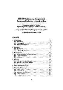
Fig. 1: Illustration of kernel-based interpolation in two dimensions. (Upper Left) Mapping of the moving image (v) to the transformed image (u). (Upper Right) A single transformed image point is computed based on a neighborhood of values in the moving image. (Lower) Kernels that are a function of the position in the transformed image are applied in succession along each dimension to yield the value in the transformed image at that

(

)

L ( µ* , Λ; y ) = ∑ [ y ]i log  y ( µ* , Λ )  i −  y ( µ* , Λ )  i i

= ∑yi log bi exp ( −li )  − bi exp ( −li )

(5)

i

where we have denoted the collection of the set of registration parameters for all N components as

{ }

Λ = λ ( n)

N n=1

.

(6)

We choose to employ a penalized-likelihood estimator with the following implicit form

{µˆ , Λˆ } = arg max Φ ( µ , Λ; y ) *

*

µ* , Λ

= arg max L ( µ * , Λ ; y ) − β R ( µ * ) ,

(7)

µ* , Λ

where R(·) denotes a penalty function that discourages overly noisy images. We refer to the implicit estimator in (7) as the “known-component reconstruction” (KCR) approach. This estimator jointly approximates both the anatomical background and the set of registration parameters associated with each known component. While the regularization term is general, we will use a pairwise quadratic roughness penalty denoted as

([ µ ] − [ µ ] ) . 2

R ( µ* ) = ∑ ∑ j k∈N

* j

* k

(8)

j

where Nj denotes a first-order neighborhood of voxels around voxel j. Note that this penalty is applied only to the background anatomy image (µ*), and there is no smoothing between the known components and the anatomy, but there is potential smoothing across the voxels in µ* that are masked by the transformed s(n) in (4). These values are ultimately replaced by µI(n) to form the reconstructed image µ.

3

C. Transformation Operator The joint estimator in (7) requires the transformation operator, W, found in (4) to be specified. The formulation in (4) is general and the transformation could potentially represent warping operations or other forms of parameterized deformations. Similarly, W could represent component transformations that have constrained motions like pivots or hinge points. In this paper we focus on the case of rigid transformations. Transformation operators associated with registration of a “moving” image to a “fixed” image can often be decomposed into two parts: 1) a mapping of gridded points in the moving image to the positions of those points in the transformed image; and 2) an interpolation operation that uses a neighborhood of voxels about each point in the moving image to generate a voxel value in the transformed image. For a 3D rigid transformation, we may denote the mapping of points from the moving image to the transformed image as   x j   xc    xc − xT   x ′j         (9)   y ′j  = Rx (θ ) R y (ψ ) Rz (φ )   y j  −  yc   +  yc − yT  ,          z ′j    z j   z c    z c − zT  T where [xj, yj, zj] represents a voxel location in the moving image, and [x'j y'j z'j]T is the position in the transformed image. The vector [xc yc zc]T is the location of the center of the image volume and [xT yT zT]T are translation parameters. The parameterized matrices Rx(θ), Ry(ψ), and Rz(φ) apply rotations about each axis with θ, ψ, and φ denoting angular values for each rotation. Thus, we may now explicitly define the six element parameter vector for transformation as λ=[xT yT zT θ ψ φ]T. While (9) denotes the mapping of the jth voxel position from [xj yj zj]T to [x'j y'j z'j]T, we recognize that the entire mapping is defined by the three “moving image” vectors x, y, and z, and the three “transformed image” vectors x', y', and z'. That is, these vectors represent the collections of all grid points in the moving and transformed images. With the point mapping defined, it remains to define the interpolation step. We consider a kernel-based interpolation approach that is separable in each dimension. An example 2D kernel-based interpolation is illustrated in Fig. 1. For each location, j, in the transformed image, a kernel is applied to a neighborhood of points in the moving image to approximate the value in the transformed image. One-dimensional (1D) (position-dependent) kernels, kj(t), are applied successively along each dimension in the neighborhood and are summed, so that each pass reduces the dimension by one – for example, in 2D, two 1D kernels applied to get a single voxel value. In 3D, three 1D kernels are used. The application of the kernels illustrated in Fig. 1 to obtain all interpolated points in the transformed image may be represented mathematically in a compact form as

u = W ( λ ) v = K z ( z′ ) K y ( y′ ) K x ( x′) v,

(10)

where u and v are vectors denoting the transformed and moving images, respectively. The K operators represent the 1D kernel applications in each direction for all locations and

IEEE TMI-2012-0258

IN PRESS

are a function of the particular point mapping. Specifically, if a four-pixel neighborhood 1D kernel is used for each dimension and both u and v have p voxels, the Kx operator applies a local kernel in the x-direction for each interpolation position to obtain vector of length 16p. The Ky operator applies a ydirection kernel to these 16p elements to obtain a vector of length 4p, and the final Kz operator uses these 4p elements and a z-direction kernel to obtain the length p vector that is the transformed image, u. It remains to define the particular kernels, k(t), used at each interpolation location. While there are many kernel choices, we employed a B-spline kernel [29] defined as follows: 2 1 2  3 − 2 t (2 − t  3  1 k (t ) =  (2 − t )  6 0   

)

t 0

2

[k ] i

[k ] i

[k ] i

)

(18)

+

ti[ k ] = 0

where the superscript [k] denotes the value at the kth iteration, ci denotes the curvature of the paraboloidal surrogate, and [·]+ denotes a function to ensure nonnegativity (truncation at zero). The first and second derivatives of g, denoted gɺ and gɺɺ , respectively, are straightforward to compute from (16) and (17). While the surrogates in (18) may be used to form an overall surrogate for the log-likelihood, we apply the convexity trick of De Pierro [47] that was also used in [33],   b  qi [ Bµ* ]i ; ti[ k ] = qi  ∑ α ij  ij µ* j − µ*[ kj ] + ti[ k ]  ; ti[ k ]   i   α ij    (19)

(

)

(

)

b  ≥ ∑ α ij qi  ij µ* j − µ*[ kj ] + ti[ k ] ; ti[ k ]   α ij  i   where bij are elements of the modified system matrix B, to obtain separable surrogates b  Q j µ* j ; µ*[ k ] ≜ ∑ α ij qi  ij µ* j − µ*[ kj ] + ti[ k ] ; ti[ k ]   α ij  i   (20)

(

(

)

)

(

(

)

)

L ( µ* , Λ; y ) ≥ ∑ Q j µ* j ; µ*[ k ] , j

where we choose . Thus, for an unregularized objective, we may apply the following updates

IEEE TMI-2012-0258

IN PRESS

µ*[ kj +1] = arg max Q j ( µ* j ; µ*[ k ] ) µ* j ≥ 0

  bij gɺ i[ k ] ti[ k ] ∑ i =  µ*[ kj ] +     bij  ∑ bij  ci[ k ] ti[ k ] ∑  i  j 

( )

( )

      +

(21)

VI. ACKNOWLEDGMENT The authors wish to thank DePuy Spine, Inc. (US and Switzerland) for providing CAD models of pedicle screws for this work. Research supported in part by the National Institutes of Health R01-CA-127444. REFERENCES [1]

[2] [3]

[4]

[5]

[6]

[7]

[8]

[9] [10]

[11]

[12] [13]

[14]

[15]

[16] [17]

B. De Man, et al., "Metal streak artifacts in X-ray computed tomography: A simulation study," IEEE Trans Nuclear Science, vol. 46, pp. 691-696, 1999. J. F. Barrett and N. Keat, "Artifacts in CT: recognition and avoidance," Radiographics, vol. 24, pp. 1679-91, Nov-Dec 2004. S. D. Stulberg, et al., "Monitoring pelvic osteolysis following total hip replacement surgery: an algorithm for surveillance," J Bone Joint Surg Am, vol. 84-A Suppl 2, pp. 116-22, 2002. L. T. Holly and K. T. Foley, "Three-dimensional fluoroscopy-guided percutaneous thoracolumbar pedicle screw placement. Technical note," J Neurosurg, vol. 99, pp. 324-9, Oct 2003. M. Y. Wang, et al., "Reliability of three-dimensional fluoroscopy for detecting pedicle screw violations in the thoracic and lumbar spine," Neurosurgery, vol. 54, pp. 1138-42; discussion 1142-3, May 2004. B. Daly, et al., "Percutaneous abdominal and pelvic interventional procedures using CT fluoroscopy guidance," AJR Am J Roentgenol, vol. 173, pp. 637-44, Sep 1999. B. De Man, et al., "Reduction of metal steak artifacts in X-ray computed tomography using a transmission maximum a posteriori algorithm," IEEE Trans Nuclear Science, vol. 47, pp. 977-981, 2000 2000. G. H. Glover and N. J. Pelc, "An algorithm for the reduction of metal clip artifacts in CT reconstructions," Med Phys, vol. 8, pp. 799-807, Nov-Dec 1981. W. A. Kalender, et al., "Reduction of CT artifacts caused by metallic implants," Radiology, vol. 164, pp. 576-7, Aug 1987. H. Li, et al., "Metal artifact suppression from reformatted projections in multislice helical CT using dual-front active contours," Med Phys, vol. 37, pp. 5155-64, Oct 2010. D. D. Robertson, et al., "Total hip prosthesis metal-artifact suppression using iterative deblurring reconstruction," J Comput Assist Tomogr, vol. 21, pp. 293-8, Mar-Apr 1997. G. Wang, et al., "Iterative deblurring for CT metal artifact reduction," IEEE Trans Med Imaging, vol. 15, pp. 657-64, 1996. O. Watzke and W. A. Kalender, "A pragmatic approach to metal artifact reduction in CT: merging of metal artifact reduced images," Eur Radiol, vol. 14, pp. 849-56, May 2004. B. P. Medoff, et al., "Iterative Convolution Backprojection Algorithms for Image-Reconstruction from Limited Data," Journal of the Optical Society of America, vol. 73, pp. 1493-1500, 1983. J. Rinkel, et al., "Computed tomographic metal artifact reduction for the detection and quantitation of small features near large metallic implants: a comparison of published methods," J Comput Assist Tomogr, vol. 32, pp. 621-9, Jul-Aug 2008. K. Lange, "Convergence of EM image reconstruction algorithms with Gibbs smoothing," IEEE Trans Med Imaging, vol. 9, pp. 439-46, 1990. T. Hebert and R. Leahy, "A generalized EM algorithm for 3-D Bayesian reconstruction from Poisson data using Gibbs priors," IEEE Trans Med Imaging, vol. 8, pp. 194-202, 1989.

13

[18] J. B. Thibault, et al., "A three-dimensional statistical approach to improved image quality for multislice helical CT," Med Phys, vol. 34, pp. 4526-44, Nov 2007. [19] J. Wang, et al., "Iterative image reconstruction for CBCT using edgepreserving prior," Med Phys, vol. 36, pp. 252-60, Jan 2009. [20] G. H. Chen, et al., "Prior image constrained compressed sensing (PICCS): a method to accurately reconstruct dynamic CT images from highly undersampled projection data sets," Med Phys, vol. 35, pp. 6603, Feb 2008. [21] J. Stayman, et al., "Penalized-likelihood reconstruction for sparse data acquisitions with unregistered prior images and compressed sensing penalties," in SPIE Medical Imaging, 2011. [22] J. A. Fessler, "Optimization transfer approach to joint registration/reconstruction for motion-compensated image reconstruction," presented at the ISBI, 2010. [23] M. Jacobson and J. A. Fessler, "Joint estimation of image and deformation parameters in motion-corrected PET," in Proc. IEEE Nuc. Sci. Symp. Med. Im. Conf., 2003, pp. 3290-3294. [24] S. Y. Chun and J. A. Fessler, "Joint image reconstruction and nonrigid motion estimation with a simple penalty that encourages local invertibility.," in Proc. SPIE 7258, Medical Imaging 2009: Phys. Med. Im., 2009, p. 72580U. [25] J. W. Stayman, et al., "Likelihood-based CT Reconstruction of Objects Containing Known Components," in Int’l Mtg. Fully 3D Image Recon., Potsdam, Germany, 2011, pp. 254-7. [26] D. L. Snyder, et al., "Deblurring subject to nonnegativity constraints when known functions are present with application to objectconstrained computerized tomography," IEEE Trans Med Imaging, vol. 20, pp. 1009-17, Oct 2001. [27] R. J. Murphy, et al., "Pose estimation of known objects during transmission tomographic image reconstruction," IEEE Trans Med Imaging, vol. 25, pp. 1392-404, Oct 2006. [28] J. F. Williamson, et al., "Prospects for quantitative computed tomography imaging in the presence of foreign metal bodies using statistical image reconstruction," Med Phys, vol. 29, pp. 2404-18, Oct 2002. [29] P. Thevenaz, et al., "Interpolation revisited," IEEE Trans Med Imaging, vol. 19, pp. 739-58, Jul 2000. [30] D. G. Luenberger, Linear and nonlinear programming, 3rd ed. New York: Springer, 2007. [31] D. C. Liu and J. Nocedal, "On the Limited Memory BFGS Method for Large-Scale Optimization," Mathematical Programming, vol. 45, pp. 503-528, Dec 1989. [32] H. Erdogan and J. A. Fessler, "Monotonic algorithms for transmission tomography," IEEE Trans Med Imaging, vol. 18, pp. 801-14, Sep 1999. [33] H. Erdogan and J. A. Fessler, "Ordered subsets algorithms for transmission tomography," Phys Med Biol, vol. 44, pp. 2835-51, Nov 1999. [34] R. L. Siddon, "Fast calculation of the exact radiological path for a threedimensional CT array," Med Phys, vol. 12, pp. 252-5, Mar-Apr 1985. [35] Y. Long, et al., "3D forward and back-projection for X-ray CT using separable footprints," IEEE Trans Med Imaging, vol. 29, pp. 1839-50, Nov 2010. [36] J. H. Siewerdsen, et al., "Volume CT with a flat-panel detector on a mobile, isocentric C-arm: Pre-clinical investigation in guidance of minimally invasive surgery," Medical Physics, vol. 32, pp. 241-254, Jan 2005. [37] S. Schafer, et al., "Mobile C-arm cone-beam CT for guidance of spine surgery: Image quality, radiation dose, and integration with interventional guidance," Medical Physics, vol. 38, pp. 4563-4574, Aug 2011. [38] C. R. Vogel and M. E. Oman, "Fast, robust total variation-based reconstruction of noisy, blurred images," IEEE Trans Image Process, vol. 7, pp. 813-24, 1998. [39] X. Pan, et al., "Why do commercial CT scanners still employ traditional, filtered back-projection for image reconstruction?," Inverse Probl, vol. 25, p. 1230009, Jan 1 2009. [40] E. Y. Sidky and X. Pan, "Image reconstruction in circular cone-beam computed tomography by constrained, total-variation minimization," Phys Med Biol, vol. 53, pp. 4777-807, Sep 7 2008.

IN PRESS

IEEE TMI-2012-0258

[41] B. De Man, et al., "An iterative maximum-likelihood polychromatic algorithm for CT," IEEE Trans Med Imaging, vol. 20, pp. 999-1008, Oct 2001. [42] I. A. Elbakri and J. A. Fessler, "Statistical image reconstruction for polyenergetic X-ray computed tomography," IEEE Trans Med Imaging, vol. 21, pp. 89-99, Feb 2002. [43] I. A. Elbakri and J. A. Fessler, "Segmentation-free statistical image reconstruction for polyenergetic x-ray computed tomography with experimental validation," Phys Med Biol, vol. 48, pp. 2453-77, Aug 7 2003. [44] S. Srivastava and J. A. Fessler, "Simplified statistical image reconstruction algorithm for polyenergetic X-ray CT," 2005 IEEE Nuclear Science Symposium Conference Record, Vols 1-5, pp. 15511555, 2005. [45] W. Zbijewski, et al., "CT Reconstruction Using Spectral and Morphological Prior Knowledge: Application to Imaging the Prosthetic Knee," in The Second International Conference on Image Formation in X-Ray Computed Tomography, Salt Lake City, UT, 2012. [46] J. W. Stayman, et al., "Model-based Reconstruction of Objects with Inexactly Known Components," in SPIE Medical Imaging, San Diego, CA, 2012, pp. 83131S-1 - 6. [47] A. R. De Pierro, "On the relation between the ISRA and the EM algorithm for positron emission tomography," IEEE Trans Med Imaging, vol. 12, pp. 328-33, 1993.

14