John L. Hennessy and David A. Patterson. Computer architecture: a quan- ... [McM92] Kenneth L. McMillan. Symbolic Model Checking:An approach to the state.
Model Checking Concurrent Assembly Algorithms Joseph Cordina, Stephen Fenech, and Gordon J. Pace Department of Computer Science, University of Malta
Abstract. Model checking has been used in various domains, to enable automatic verification of properties for a given model. Especially in cases when the correctness of the the model is not evident due to the complex nature of the description, model checking can be an indispensable tool. One such domain is the use of concurrent assembly algorithms for lowlevel synchronisation, which can be notoriously difficult to check their correctness or even test. In this paper we look at this domain, and explore the use of model-checking in verifying a number of such algorithms, such as barrier synchronisation and wait-free CSP channel communication. We tackle the state explosion problem inherent in model checking by making use of abstraction techniques to remove rendundant information in the the model, and partial-order techniques to remove redundant interleavings of actions. Finally, we also investigate the use of structural induction to reason about families of systems of arbitrary size. Making use of symmetry and induction, we verify algorithms with an unbounded number of identical participating tasks.
1
Introduction
Model checking has been extensively used in the verification of complex systems. In critical systems, analysis of properties along all possible execution paths makes it an attractive alternative to testing and simulation. In the field of asynchronous concurrent algorithms, building testing suites with high state-space coverage can be particularly challenging, since concurrency may introduce different interleavings which are difficult to control through the testing suite. In this paper, we present our recent results in the verification of concurrent wait-free assembly algorithms through the use of standard model checking techniques. We look into algorithms running on three different shared memory architectures: Single Processor, Symmetric Multi-Processor (SMP) and Asymmetric Multi-Processor (ASMP), with the main focus on the ASMP. In the SMP architecture, the processors are identical and share the same clock so they are synchronised [HP02]. On the other hand the ASMP architecture does not have such a constraint and thus we cannot know how long an instruction will take to execute on different processors. In particular, we look into wait-free algorithms used in the core of the KRoC Occam compiler [WW96], to handle communication between different threads. As with most real-life applications of model checking, the main challenge is
primarily that of controlling the state explosion problem. Due to the multiple interleavings that are possible in such algorithms, the state space grows very quickly. The second challenge is that of reasoning about parametrised systems. Rather than the verification of a stand-alone program, most of the algorithms used may interact with any number of other programs. For example, the resolution of channel synchronisation in a CSP-like domain may have any number of readers trying to take the data provided by the writer. We present structural induction techniques to reason about such families of systems using model checking. In this paper we present the application of these techniques for the verification of the algorithms used internally by KRoC to handle thread barrier synchronisation and channel communication using wait-free algorithms [Vel98]. In both cases, we use inductive reasoning with model checking to prove the correctness of the algorithms for any number of processes taking part in the synchronisation.
2
Background
A Kripke structure is a tuple M = hQ, I, t, vi, where Q is a finite set of states, I ⊆ Q is a set of initial states, t ⊆ Q × Q is a total transition relation between states and v ∈ Q → 2A is a valuation function over a set of atomic propositions A. The valuation function v corresponds to which propositions hold in which states. We say that proposition p ∈ A holds in state q ∈ Q in M , written q |=M p, if p ∈ v(q). We extend this notation for boolean expressions. q |=M e ∧ f holds if both q |=v e and q |=v f . Similarly, we define the other boolean operators. The set of valid paths in a Kripke structure M are infinite sequences of states σ ∈ seq(Q) such that σ0 ∈ I and for all i, (σi , σi+1 ) ∈ t, where the subscript is the index of the path. Linear Time Logic (LTL) is used to reason about properties along such paths. An LTL formula is either a boolean expression over atomic variables, or uses the temporal operators G, F, X and U. The semantics of LTL over a path σ, are defined as follows (σ +i corresponds to the path identical to σ but dropping the first i initial items): df
σ |=M e
= σ0 |=M e
σ |=M X p
= σ +1 |=M p
σ |=M F p
= ∃i · σ +i |=M p
σ |=M G p
= ∀i · σ +i |=M p
df
df
df
df
′
σ |=M p U q = ∃i · σ +i |=M q and ∀i′ < i · σ +i |=M p A Kripke structure M is said to satisfy LTL formula e, written as M |= e, if all valid paths in M satisfy e. Linear Time Logic without next-time operator (LTL/X) is identical to LTL, except that X may not appear in properties.
3
Modelling
We model concurrent algorithms running on any of three different shared memory architectures: Single Processor, Symmetric Multi-Processor (SMP) and Asymmetpc=2 zf=1 pc=2 zf=0 pc=2 zf=0 [1]=0 [1]=1 [1]=0 ric Multi-Processor (ASMP). In the SMP architecture, the processors are identical pc=3 zf=1 and share the same clock so they are syn[1]=0 chronised [HP02]. On the other hand the ASMP architecture does not have such a pc=4 zf=1 [1]=0 constraint and thus one cannot know how long an instruction will take to execute on pc=5 zf=1 [1]=1 different processors. This can be modelled by giving each instruction the possibility Fig. 1: Part of the Kripke structure to stutter so in this way an instruction of the mutual exclusion algorithm. may take any amount of time to finish. The dotted transitions correspond This also resolves the problem of knowing how many cycles each instruction takes, to the other external process. since the model will cover any number of cycles. In our model, the data and code will be assumed to reside in different memory areas. Furthermore, the programs will not have access to write to the code memory areas — in other words, we will be looking at static (non-self modifying) algorithms. pc=1 zf=1 [1]=0
pc=1 zf=0 [1]=0
pc=1 zf=0 [1]=1
pc=1 zf=1 [1]=1
Algorithms are given a semantics in terms of a Kripke structure, with the states consisting of the data stored in the registers (including program counters) and the memory. The transition relation is based on the semantics of the assembly instruction found in memory at the location pointed to by the program counter. To reduce the model to a reasonable magnitude, only the memory locations used in the algorithms will be modelled. 1 2 3 4 5
spin :
cmp [1] 0; jne spin ; noop ; // Crit . Sec . mov [1] 1; jmp spin ;
spin :
cmp [1] 1; jne spin ; noop ; // Crit . Sec . mov [1] 0; jmp spin ;
Listing 1.1: Mutual exclusion try For instance, consider the two concurrent programs shown in listing 1.1. Both processes use memory location 1 in order to provide mutual exclusion. The state space will be made up of all the possible values of the memory location 1 and the value of the registers used (the program counters of the two processes pc1 and pc2 and their equality, or zero flags). Figure 1 shows a small part of the reachable states of the Kripke structure derived from this program.
3.1
Formal Semantics of Assembly Programs
Based on the model we derive, one can try to verify that the algorithm actually guarantees mutual exclusion between the two concurrent processes — it is never the case that both processes will be in the critical section at the same time. This can be specified as the LTL property as G(¬(pc1 = 3 ∧ pc2 = 3)). In table 1, one can find the operational semantics given to some typical assembly instructions. The transitions are between triples (r , lm, gm) — with the information stored in the registers, local memory and global memory respectively. All transitions are labelled by two parameters (−→M prg ), the program being given a semantics, and the set of locations in global memory that are updated by the instruction. We call transitions with M = ∅, local transitions. In the case of parallel composition, the global memories are merged based on this latter parameter. Based on these semantics, we can give a Kripke structure ′ interpretation to a program prg, with q −→ q ′ being defined as ∃M · q −→M prg q . We refer to this as [[prg]]. Lemma 1. Any sequence of local transitions does not change the global memory component of the state: If (r, lm, gm)(−→∅prg )∗ (r′ , lm′ , gm′ ), then gm = gm′ . The proof follows by induction on the number of transitions taken, and the basic definitions of instruction semantics. The state explosion problem unfortunately limits the size of the model which can be model checked in a tractable amount of time [EMCJ99]. Many techniques have been devised in order to be able to enable model checking of larger systems. We will now explain some domain specific optimisation we performed on the models produced. The state space described in the semantics is simply far too big to handle using model checking. One of the main culprits is the fine-grain instructions, introducing far too many interleavings. Despite the fact that unless the global memory is modified, there is no interaction between concurrent programs, the semantics keeps account of all the individual instructions carried out in each thread. To relieve this problem, we introduce a less fine grained semantics, giving an abstraction of the original system, which collapses redundant individual instructions together. We define =⇒M prg to be defined for sequential programs for any sequence of instructions not communicating with the global memory, followed by a single instruction that does or a loop which does not modify the global state: df
′ ′ ′ (r , lm, gm) =⇒M prg (r , lm , gm ) = ′ (r (pc) = r (pc) ∧ M = ∅ ∧ (r , lm, gm)(−→∅prg )∗ (r ′ , lm ′ , gm ′ )) ′ ∅ ∗ ′ ′ ∨ (r , lm, gm)(−→M prg ◦ (−→prg ) )(r , lm , gm )
Furthermore, we constrain the states of the automata to the initial states, the destinations of global transitions and jump instruction locations which enable a local loop. We can use this rule to induce more compact sequential program
Sequential program semantics: prg[r (pc)] = noop (r , lm, gm) −→∅prg (r [pc := r [pc + 1]], lm, gm) prg[r (pc)] = mov [m] n {m} (r , lm, gm) −→prg (r [pc := r [pc + 1]], lm, gm[m := n]) prg[r (pc)] = jmp n (r , lm, gm) −→∅prg (r [pc := n], lm, gm) prg[r (pc)] = jeq n ∧ r (eq) (r , lm, gm) −→∅prg (r [pc := n], lm, gm) prg[r (pc)] = jeq n ∧ ¬r (eq) (r , lm, gm) −→∅prg (r [pc := r [pc + 1]], lm, gm) Stuttering: (r , lm, gm) −→∅prg (r , lm, gm) Parallel composition: ′ ′ ′ 1 (r 1 , lm 1 , gm) −→M prg1 (r 1 , lm 1 , gm 1 ) M2 ′ ′ (r 2 , lm 2 , gm) −→prg (r 2 , lm 2 , gm ′2 ) 2 1 ∪M2 ((r 1 , r 2 ), (lm 1 , lm 2 ), gm) −→M prg1 kprg2 ((r ′1 , r ′2 ), (lm ′1 , lm ′2 ), merge((gm ′1 , M1 ), (gm ′2 , M2 ))
Table 1: Semantics of assembly programs
semantics, using the stuttering and composition rules to define a more compact semantics for concurrent programs. We will refer to such semantics of a program prg, as [[prg]]A . Theorem 1. Given a program prg, and an LTL/X formula π in which basic propositions refer only to the global memory, [[prg]] |= π if and only if [[prg]]A |= π. The proof follows in a straightforward manner using structural induction on the temporal properties, and the fact that the leaf properties change only after a global transition (lemma 1). Furthermore, local loops are maintained in the abstract system, ensuring that deadlocks are not lost. The result of this theorem can be extended to allow the LTL/X formula to refer to program counter values at the end of a global memory access. In practice, the abstraction reduces the reachable state space drastically. Furthermore, after collapsing such chains of instructions, we can also syntactically look at the program and identify registers and local memory locations which no longer have an affect on the execution of the program. Since we use a symbolic model checker, we prune out such state variables to reduce the state space of the resulting system even further. 3.2
Reasoning about Families of Processes using Induction
One problem with most algorithms at the core of a compiler, is that the interaction is not strictly between a fixed number of processes. For instance, if one looks at a multi-way synchronisation algorithm, it should work regardless of the number of participating entities. Similarly, in the case of channel communication in Occam, one can have one single writer, and multiple reader competing for the channel. In both these examples, the problem is to prove that a system satisfies a property for any number of processes. For a property π, the property one would like to verify is of the form: ∀n · [[QkP n ]] |= π To prove this property for any number of copies of P , one can use an inductive approach, by taking the weakest process α satisfying π, and proving that (i) Q |= π; and (ii) αkP |= π. The first property can be easily verified using the techniques already presented. The second is more difficult to prove, since we need to be able to generate α. One possibility is to consider the system with a chaotic system for α (chaotic in that it can perform any action), and constrain the model checking tool to work on paths for which α satisfies π. In general this is not straightforward to do, but by limiting ourselves to safety properties expressed as observers [HLR94], which take the input and output of the system and return one output stating whether or note the system is running correctly, we can reason about the weakest system directly, proving that if the observer running on the chaotic system has always been true in the past, the observer of the global system will also be true. In this manner, we enable reasoning about whole families of systems. chaoskP |= G (observer(chaos) ⇒ observer(chaoskP ))
4
Case Studies
In this section we will look into a number of case studies we will verify using the techniques described in this paper. 4.1
Thread Barrier Synchronisation
Barrier synchronisation algorithms are widely used when a job is split between a number of processes which then wait for each other to finish in order to agglomerate the results. This algorithm makes use of two semaphores and two different threads to do the synchronisation. With k threads to synchronise, k − 1 threads will signal on a semaphore A followed by waiting on semaphore B. The remaining thread (referred to as the asymmetric thread) tries to cancel the effect of the other threads by waiting for k − 1 times on A then signaling semaphore B for k − 1 times freeing the other threads waiting on this semaphore. Using this model we model check that all the threads eventually reach the barrier before any continue any further. Applying abstraction meant a reduction of state variables by an average of 18%, enabling us to verify the algorithm for up to 10 processes taking less than 15 minutes. 4.2
Generalised Thread Barrier Synchronisation
Induction cannot be applied directly to the model just described, since the semaphore location needs to be to hold a value of up to k, for a general value k. The solution we adopt, is that we encode the semaphore location and the asymmetric thread into a single module. When, in the algorithm, one adds a new thread, one also has to add a new wait to the asymmetric thread and a new signal at the end. In order to model this we are going to create a number of components. Module SemA will take two signals as input which outputs true once both have been received. SemA models the part of the asymmetric thread which waits on semaphore A. Module SemB models semaphore B and the part of the asymmetric thread which signals on semaphore B in order to free the symmetric threads. The symmetric thread is modelled as module P and has three states: the signaling state where it signals semaphore A; the waiting state where the thread waits on semaphore B; and the ready state. Figure 2 shows the interaction between the modules. In order to add another thread, one needs to add more symmetric threads and cascade the semaphore modules. Here, the ready signal from the first SemA is directed to Signal1 of the second thus the final SemA module will issue the ready only when signals have been sent to all the semaphores. This is then directed to the SemAReady of the SemB modules. For this proof, a number of observers are used. One observer checks that it receives all the signals before receiving the wait requests. Furthermore, another observer checks that each signal/wait is received only once.
SemA Signal1 Signal2 Ready
Observer signal1 signal2 wait1 wait2 Ok
SemB SemAReady waitreq1 wait1 waitreq2
Always ok
SemA
P1
Signal1
Signalling
SemB
Signal2
Waiting
SemAReady
Ready
Signal1
Ready
waitreq1
Signal2
P2
waitreq2
SemA
Ready
wait1
SemAReady
P3
waitreq2
wait1 wait2 ready
wait2
Waiting
Waiting
ready
Ready
Fig. 2: P 1 and P 2 are two symmetric threads, whilst the asymmetric thread is encoded in SemA and SemB
SemB waitreq1
Signalling
Signalling Ready
wait2 ready
Observer signal1 signal2 wait1 wait2 Ok
Fig. 3: Inputs to SemA1 and SemB1 are now unbound and thus SMV will assign them a value nondeterministically. Observer1 will be used to control the inductive assumption.
With these observers in place, for the base case, all one needs to model check is that their output is always true. For the inductive case (Figure 3), we leave the modules to work in a nondeterministic manner (representing the behaviour of the k processes), and add another unit (as the (k + 1)th process). Two instances of the observers will be used to monitor the behaviour of the blocks inside (outputting okk ), and that of the overall system (outputting okk+1 . By thus need to show that restricting the behaviour of the k processes to satisfy the property, the global system still satisfies the property: G (always okk ⇒ okk+1 ) (where always okk checks whether okk was always true in the past). Using this approach, we model check the correctness of thread barrier synchronisation for any number of communicating processes. 4.3
Wait-Free CSP Channel Communication
In this case study we look at, and model check Vella’s wait-free CSP channel algorithm for shared memory multiprocessors [Vel98]. This algorithm is used in the kernel of the KRoC [WW96] Occam compiler. Wait-free algorithms offer various advantages over locking algorithms but they are typically intricate algorithms, difficult to develop and to confirm their correctness under all possible interleavings. We first present simple channel communication in order to get a grasp of the basic algorithm followed by alternate channel communication. In the CSP model of concurrency two processes may communicate only through blocking and uni-directional channels. Simple Channel Communication In the simple channel communication the inputting and outputting tasks have three shared memory locations; the channel word, input workspace and output workspace. The channel word will store the workspace’s address of the task which has committed itself to the communication. The output workspace will store the output value whilst the input
workspace is where the value is stored once received. The output task will behave similarly to the input task seen in listing 1.2. Swap InputWorkspac e location into the channel word ; if channel word was 0 { Sleep ; ( wait for output task to arrive to same point ) } else ( output task is already waiting ) { Reset the channel word to 0; Copy value from OutputWorksp ac e to InputWorkspa ce ; Wake the output task ; }
Listing 1.2: Pseudocode of channel communication (input task) This algorithm can be modelled directly using the translation we have given, and we verify that (i) the algorithm never deadlocks (the tasks always finish); and (ii) that channel communication is always successful (the correct value is transferred from the output to the input workspace). Alternate Channel Communication In the alternate channel communication, a single inputting task receives an input from a number of channels — corresponding to (a1 .P1 + a2 .P2 . . . + an .Pn ) | a ¯1 .Q1 | a ¯2 .Q2 . . . | a ¯n .Qn An additional memory location which in [Vel98] is referred to as a Pointer is used to hold the state of the input task. An outputting task will behave mainly like in the single channel communication except that when it finds the address of the inputting workspace it has to inform the inputting task by swapping READY into the Pointer (listing 1.3). Swap OutputWorksp ac e location into the channel word if channel word was 0 { Sleep ( wait for input task to arrive to same point ) } else ( input task is waiting or still enabling ) { Swap READY into Pointer if pointer was WAITING ( input task is sleeping ) { Wake input task ; } Sleep ; }
Listing 1.3: Pseudocode of alternate channel communication (output task) The input task (listing 1.4) starts by enabling the channels. Once the enabling is ready it will swap WAITING into the pointer. If the value was still ENABLING it can safely go to sleep. If on the other hand it was READY, it means that an output task has committed itself so the disabling phase will follow. Since we have already swapped WAITING into the pointer, we need to set it back to READY. This
for every channel ( Enabling phase ) { Swap InputWorkspa ce location into channel ; if channel was not 0 { set Pointer to READY ; restore channel word to previous value ; } } Swap WAITING into Pointer ; if Pointer was Ready { Swap READY back into Pointer ; if Pointer had become Ready anyway { Sleep ; } } else it is ENABLING { Sleep ; } for every channel ( Disabling phase ) { Swap 0 into channel if channel was not InputWorkspa ce location { restore channel word to previous value ; store channel id in order to read from this channel ; } } Reset the channel word to 0; Copy value from chosen OutputWorksp a ce to InputWorkspa c e ; Wake the corresponding output task ;
Listing 1.4: Pseudocode of alternate channel communication (input task)
is not done atomically thus an output task may mistakenly read that the input task was in the WAITING state. We can identify such a situation by swapping READY into the pointer. If it is still WAITING it means that no output task has read this value, so we can continue normally. If not, we simply go to sleep and leave it up to the output task to reawaken the inputting task. Once the communication occurs the input task will disable the channels and then obtain the value directly from the output workspace and then wake the output task. Modeling the algorithm Abstractions are used to simplify the algorithm thus making the problem tractable. Rather than storing the workspace address in the channel word it is sufficient to store a single value storing one of three possible values: (i) the input task has committed; (ii) an output task committed; (iii) no task has yet committed. Despite the abstractions used, the model obtained was still too large to reason about. The solution we adopted was to abstract further from the implementation, reducing the state variables by an extra 80%, but separately model check that this abstraction is correct. Using the abstracted model we verified the following properties for up to six output tasks running in parallel: 1. If the processes loop, to input (and output) repeatedly, the input process will terminate infinitely often, implying that the algorithm introduces no deadlock. 2. It is never the case that every task is sleeping. 3. Every output task may output — although the algorithm does not deal about starvation, and an output process may never manage to output, there is always a possibility (path in the state graph in which) it manages to do so. 4. The communication is sound — once an output task is chosen, the correct value will be transferred to the input task. 5. No output is lost. 4.4
Wait-Free CSP channel Communication with an Arbitrary Number of Output Processes
Induction was approached in a similar manner as in Section 4.2. We first identify elements (both memory and code) that need to be replicated for every output task that is added. The main issues was the enabling and disabling of channels and the shared access to the pointer value since we will have an unknown number of channels. These were defined recursively as a number of communicating modules thus abstracting away from threads and processors. Using this model we proved that given any number of outputting processes (i) the input task will repeatedly receive inputs from the output tasks and will never end up in a deadlock; and (ii) an output task may eventually perform an output even when running in parallel with an unbounded number of output
tasks (an output task may never be chosen to output since the algorithm does not ensure fairness). We made use of a number of assumptions in order to prove these properties: (i) both the enabling and disabling phase terminate; and (ii) the tasks will eventually gain access to the pointer value. These assumptions were needed since we generalise how many output processes are running.
5
Conclusions and Future Perspectives
In this paper, we have looked into the application of model checking techniques for the analysis of compiler-kernel wait-free algorithms used in the KRoC Occam compiler. We have presented different techniques for state space reduction including abstraction and partial-order analysis. We have also used structural induction techniques for the verification of families or networks of processes, to ensure that the compiler-kernel algorithms work well for any number of interacting processes. These techniques have been developed into a tool, which uses SMV as a back-end for verification. It has been applied on a number of algorithms used in the core of the KRoC compiler, which have been verified correct. Leven et al [LME04,Meh06] look into the model checking of assembly code where instead of creating a model they make use of a virtual processor to avoid any potential errors in the translation. A similar approach to ours was taken by Basin et al [BFG03] in order to model check bytecode instructions. There is also a great deal of work concerning abstraction in order to prove properties over larger systems [CGL94]. We made use of symbolic methods of abstractions but another type of abstraction is abstract model checking as in [CC99,Gra94,Gra99]. Partial-order abstraction similar to the one employed here is also employed in StEAM [Meh06]. Structural induction, as used in our approach, has also employed in a in [McM92] and is discussed in [Jha96] as employing symmetry. In our case studies, we have looked at LTL properties of these systems. Clearly, concurrency introduces various issues which require a branching time logic to express. Certain properties, such as ‘whenever the algorithm is at location start, with register r being zero, the other thread may eventually reach location critical’, cannot be expressed in a linear time logic. We plan to look into the use of other temporal logics such as CTL and µ-calculus, to verify more properties of our systems. We have used modular verification techniques to verify networks of processes. These techniques were also useful in the abstraction of assembly code to reduce the complexity of the model checking task. However, the use of modular verification techniques was rather ad hoc, and we plan to extend our verification tool to enable management of module properties to support this form or reasoning.
References [BFG03]
David Basin, Stefan Friedrich, and Marek Gawkowski. Bytecode verification by model checking. J. Autom. Reason., 30(3-4):399–444, 2003.
[CC99]
P. Cousot and R. Cousot. Refining model checking by abstract interpretation. Automated Software Engineering, 6(1):69–95, 1999. [CGL94] Edmund M. Clarke, Orna Grumberg, and David E. Long. Model checking and abstraction. ACM Transactions on Programming Languages and Systems, 16(5):1512–1542, September 1994. [EMCJ99] Doron A. Peled Edmund M. Clarke Jr., Orna Grumberg. Model Checking. MIT Press, 1999. [Gra94] S. Graf. Verification of a distributed cache memory by using abstractions. In Workshop on Computer-Aided Verification, CAV’94, Stanford. LNCS 818, Springer Verlag, 1994. an updated version of the paper in the CAV proceedings accepted at Distributed Comput ing. [Gra99] S. Graf. Characterization of a sequentially consistent memory and verification of a cache memory by abstraction. Distributed Computing, 12, 1999. accepted for publication since 1995. [HLR94] Nicolas Halbwachs, Fabienne Lagnier, and Pascal Raymond. Synchronous observers and the verification of reactive systems. In AMAST ’93: Proceedings of the Third International Conference on Methodology and Software Technology, pages 83–96, London, UK, 1994. Springer-Verlag. [HP02] John L. Hennessy and David A. Patterson. Computer architecture: a quantitative approach. Morgan Kaufmann Publishers Inc., San Francisco, CA, USA, 2002. [Jha96] Somesh Jha. Symmetry and Induction in Model Checking. PhD thesis, School of Computer Science, Carnegie Mellon University, Pittsburgh, PA 15213, October 1996. [LME04] Peter Leven, Tilman Mehler, and Stefan Edelkamp. Directed error detection in c++ with the assembly-level model checker steam. In SPIN, pages 39–56, 2004. [McM92] Kenneth L. McMillan. Symbolic Model Checking:An approach to the state explosion problem. PhD thesis, Carnegie Mellon university, May 1992. [Meh06] Tilman Mehler. Challenges and applications of assembly level software model checking. PhD thesis, University of Dortmund, March 2006. [Vel98] Kevin Vella. Seamless Parallel Computing on Heterogeneous Networks of Multiprocessor Workstations. PhD thesis, University of Kent at Canterbury, December 1998. [WW96] David C. Wood and Peter H. Welch. The kent retargetable occam compiler. In WoTUG ’96: Proceedings of the 19th world occam and transputer user group technical meeting on Parallel processing developments, pages 143–166, Amsterdam, The Netherlands, The Netherlands, 1996. IOS Press.