method is robust, computationally efficient and achieves a high degree of segmentation ... For example, the intensity based methods are likely to fail if ... However, un- der a model-guided framework of segmentation, the exis- .... caudate nuclei from the training set. ..... feature selection problem in machine learning. Therefore ...
Model-Guided Segmentation of 3D Neuroradiological Image Using Statistical Surface Wavelet Model Yang Li, Tiow-Seng Tan Department of Computer Science National University of Singapore
Abstract This paper proposes a novel model-guided segmentation framework utilizing a statistical surface wavelet model as a shape prior. In the model building process, a set of training shapes are decomposed through the subdivision surface wavelet scheme. By interpreting the resultant wavelet coefficients as random variables, we compute prior probability distributions of the wavelet coefficients to model the shape variations of the training set at different scales and spatial locations. With this statistical shape model, the segmentation task is formulated as an optimization problem to best fit the statistical shape model with an input image. Due to the localization property of the wavelet shape representation both in scale and space, this multi-dimensional optimization problem can be efficiently solved in a multiscale and spatial-localized manner. We have applied our method to segment cerebral caudate nuclei from MRI images. The experimental results have been validated with segmentations obtained through human expert. These show that our method is robust, computationally efficient and achieves a high degree of segmentation accuracy.
1. Introduction Segmentation of anatomical structures from magnetic resonance imaging (MRI) or computed tomography (CT) data sets is the first and basic step in many medical image applications, such as diagnosis, therapy evaluation, surgical planning and navigation. Because manual segmentation is time-consuming and lacks reproducibility, the development of automated or semi-automated techniques is highly desirable. In general, the development of computer-assisted segmentation methods is challenging due to many difficulties. For example, the intensity based methods are likely to fail if the distribution of intensity values of the structure of interest overlaps with those of the surrounding structures. Moreover, in medical images, the object boundaries are often smeared due to low image contrast or even missing when blended with other surrounding structures with similar in-
Ihar Volkau, Wieslaw L. Nowinski Biomedical Imaging Lab Singapore Bioimaging Consortium
tensity values. Therefore, boundary-based methods such as “snake” [6] may “leak” and result in a poor segmentation. To overcome these difficulties, a model with a prior knowledge of the target object can be very helpful. However, under a model-guided framework of segmentation, the existence of variability of object shape requires that the shape model used should be in a statistical form. A number of statistical shape models as indicated in the next few paragraphs have been proposed for this purpose. In the Active Shape Model (ASM) [4] approach, a shape is represented by using the point distribution model (PDM). From a training set, a mean shape is formed from the mean points’ coordinates (after normalization to exclude size, orientation and position) over all members in the training set. Through the principal component analysis on the training set, eigenvectors which represent the eigen shape variation modes are computed and new shapes are modeled by the mean shape plus a linear combination of these eigenvectors. As the training set is usually small in size, relative to the dimensionality of the shape space, the possible ways to deform a shape are limited to a linear subspace of the complete shape space. Moreover, the representation of shape is composed of a set of discrete points. Thus, we know the geometry of a shape only at a finite set of points. When a high degree of precision is required on the shape, a corresponding dense sampling is needed. This shape model can be verbose and thus not efficient for computation. On the other hand, parametric modal decomposition model provides continuous and concise representation of a shape. The decomposition basis is usually a set of different frequency harmonics. The modal decomposition produces a small number of coefficients which capture the overall shape of the objects. The commonly used decomposition basis functions are Fourier [10] [11] and spherical harmonics [7]. In another perspective, these functions are periodic and globally supported (rather than localized in space), so a small perturbation in one parameter can affect the entire outline of a shape. They are thus not easy to be manipulated efficiently and effectively to describe local deformations. Moreover, when solving an optimization problem to
best fit a prior model with an input image, the basis functions are not spatial-localized, thus the coefficients in one scale (which are correlated) have to be optimized at the same time. This means that the optimization problem is complex and computationally expensive. In contrast to the Fourier and spherical harmonics, wavelet basis functions are compactly supported and have the localization property both in frequency and space. Statistical shape models based on wavelets for 2D shape were presented [3][5], where shape boundaries are explicitly parameterized into two coordinate functions and then decomposed with the first-generation wavelets that work with manifolds defined on regular grids. The rigorous requirements in this explicit parametrization are the major obstacles to extending this wavelet basis onto the work here on 3D surfaces. We need, firstly, a surface parametrization that provides the correspondences between objects in the training set. Secondly, the first-generation wavelets require the surface to be parameterized by regular grids. Since the topology of anatomical structures is usually a sphere, we need two parameters, longitude and latitude to characterize such a surface. However, in doing so, distortions are inevitably at the south and north poles. In our proposed model-guided segmentation framework, we introduce a new statistical surface wavelet model. We adopt a newly developed surface wavelet scheme [1] which can perform wavelet analysis directly on a surface mesh with subdivision mesh connectivity. This second-generation wavelet scheme can work with manifolds defined on non-regular grids, more specifically, on the Catmull-Clark subdivision mesh. Based on the shape representation using this wavelet scheme, our model represents the statistical shape information in a multiscale and spatiallocalized way. This feature is very valuable to the optimization problem to best fit a prior model with an input image as the problem can now be solved in a divide-and-conquer manner. This thus results in a more robust and efficient segmentation method. Our work here differs from the recent work on shapedriven segmentation using spherical wavelet [8]. Their work uses wavelets [9] defined on a triangulated subdivision mesh, and a different objective function (and multiscale gradient descent algorithm) in performing model-guided segmentation. Unlike theirs, our model integrates the shape variations with the variations in similarity transform (translation, rotation and scaling). Such a prior model integrating both the two kinds biological variations can be more robust than a pure shape model with separated parameters describing the similarity transform [12] [7]. The remaining part of the paper is organized as follows. Section 2 discusses the construction of a prior statistical model from a set of MRI scan data. Section 3 presents the model-guided segmentation method using our proposed sta-
tistical surface wavelets model. Next, Section 4 applies our method to segment the cerebral caudate nuclei and presents the experiment results. Lastly, Section 5 concludes the paper with possible future research directions.
2. The statistical surface wavelet model For the discussion of the proposed framework, we use the 18 MRI scans from the Internet Brain Segmentation Repository (IBSR) [14] as an example of a training set. For these MRI scans, the principal gray and white matter structures of the brain, including the right and left caudate nuclei, have been segmented. To compute a statistical surface wavelet model (Section 2.3), we first need to address the correspondence finding and re-meshing of the training set (Section 2.1). We also provide a quick review on the use of wavelet to decompose shapes (Section 2.2).
2.1. Finding the correspondence and re-meshing In building a statistical shape model, we first need to establish correspondence among the shapes in the training set. In our work, this problem is solved by using the spherical harmonics (SPHARM) normalization [2]. Figure 1 gives an example of the SPHARM normalization of a segmented cerebral lateral ventricle. After binary volumetric data is obtained through manual segmentation, the outermost facets of the voxels are extracted as the surface mesh of the object (shown in Figure 1(a)). Next, a continuous and uniform mapping from the object surface to the unit sphere is computed. The result is a bijective mapping (Figure 1(b)) between each point V(x, y, z) on the surface and two spherical coordinates θ and φ on a unit sphere. In other words, the coordinates of the points on the surface are captured as functions x(θ, φ), y(θ, φ) and z(θ, φ) defined on the unit sphere. Therefore, they can be expanded into a set of spherical harmonic basis functions and resulting in a series of coefficients. With these, translation, rotation, and scaling in objects are removed subsequently (see [2] for details) and a set of normalized SPHARM coefficients is generated. After normalization, points on two surfaces with the same spherical coordinates θ and φ are defined as corresponding pairs. To reconstruct the shape from the normalized coefficients (as shown in Figure 1(d)), we use a re-sampling grid on the unit sphere with Catmull-Clark subdivision mesh connectivity (as shown in Figure 1(c)). This subdivision connectivity is needed in our subsequent wavelet analysis. Figure 2 shows the 18 reconstructed right caudate nuclei from the training set. As mentioned, for each shape, the SPHARM normalization removes its translation, rotation and scaling, or collectively its similarity transform. As such, it also removes the correlation between the position and the shape of the anatomical structure (in the original images). It was, how-
(a)
(b)
(c)
(d)
Figure 1. Correspondence finding and re-meshing. (a) The extracted surface net. (b) Unit sphere mapping. (c) The re-sampling grid with Catmull-Clark subdivision mesh connectivity. (d) The normalized and re-meshed surface. ÿ ÿ ÿ
Figure 3. Wavelet transformation on Catmull-Clark subdivision mesh.
Figure 2. The 18 samples from the Internet Brain Segmentation Repository (IBSR).
ever, observed in [12] [7] that a prior model integrating similarity transform is much more robust than a pure “shape” model. Therefore, in our framework, we use a simple principal component alignment method to register a shape obtained from the SPHARM normalization with its original shape in the input image to restore its similarity transform information in the Talairach coordinate system [13].
2.2. Shape representation using wavelet Having solved the correspondence issue and obtained the required subdivision mesh by re-sampling, we can now perform wavelet analysis on the surface mesh directly with the scheme introduced in [1]. It is a second-generation wavelet based on the hierarchical mesh connectivity defined by Catmull-Clark subdivision. In this subdivision scheme, a mesh is subdivided from sub-mesh to super-mesh by inserting new vertices (see Figure 3 for an example). The vertices, denoted by f, e, and v, respectively in a super-mesh correspond to a face, an edge, or a vertex, respectively in the submesh. A wavelet decomposition step can be considered as an operation applied to a super-mesh, in which a sub-mesh is computed to approximate the super-mesh. The vertices, denoted by v’, on this sub-mesh represent the coefficients
of the scaling function. The shape details which are missing in the sub-mesh can also be computed and are denoted by vectors e’ and f’ which describe the differences between the approximating mesh and the super-mesh. These vectors represent, in fact, the coefficients of wavelet functions. We denote the set of all vertices contained in the mesh after j subdivisions as V (j). When we obtain a finer resolution mesh V (j + 1) through subdivision, we denote the e vertices and f vertices added to the subdivision as the vertex set W (j). The complete set of vertices in the finer resolution j+1 is V (j+1) = V (j)∪W (j). Let S be a surface and x ∈ R3 a vertex on S. Using wavelet transform described above, S can be represented by a weighted summation of a set of scaling and wavelet functions (Figure 4) defined on the surface with different scales and locations: � � � j j S(x) = wm ψm (x) + vn0 φ0n (x) (1) j≥0 m∈W (j)
n∈V (0)
where, φ0n is the scaling function of the coarsest scale at j vertex n, ψm is the wavelet function of scale j at vertex m, 0 j and vn and wm are the corresponding coefficients of these j functions. In 3D, vn0 and wm are vectors with 3 elements and each element represents one of the coordinates x, y, z. For our training set from IBSR, after decomposing the prepared surface meshes in the training set with this wavelet j scheme, we found that |wm | < 0.5mm for j ≥ 3. However, the minimum voxel size in IBSR is 0.8371mm, and we can j thus omit |wm | for j ≥ 3. Hence, we only use the first 4 scale levels, for a total of |V (0)| + |W (0)| + |W (1)| + |W (2)| = 8 + 18 + 72 + 288 = 386 coefficient vectors to describe each shape. Suppose we have N shapes in the training set. With the wavelet decomposition method de-
Then the covariance matrix of the j th coefficient vector is: Σj = (a)
(b)
(c)
Figure 4. Basis functions on a sphere. (a) Scaling function. (b) Wavelet function corresponding to an edge. (c) Wavelet function corresponding to a face.
(a)
(b)
Figure 5. (a) Mean shape. (b) Color coded shape variation distribution.
scribed above, the ith shape of the training set can be reprej T sented as: ci = [c1i , · · · , cM i ] . Here, ci , i = 1, ..., N , and th j = 1, ..., M stands for the j coefficient of the ith shape. In our case, N = 18 and M = 386.
2.3. Computing statistical shape model After decomposing the training set and using ci , i = 1, ..., N to represent the ith � shape, we can first compute N the mean shape as: c = N1 i=1 ci . Figure 5(a) shows the mean shape c of our training set. The mean shape is used as the initial guess when performing segmentation of an unknown input shape. Also, the spatial distribution of the shape deviations from the mean shape can be computed. This is shown in Figure 5(b) with different colors representing the different extent of deviations. From this figure, we can see that the tail of the caudate nucleus is the most variable part, while the middle body part is relatively stable. Because of the multiscale and spatial-localization property of wavelet basis, every wavelet coefficient vector only defines the shape at a specified scale and spatial location. Therefore, statistical analysis can be applied on every coefficient vector separately to obtain the multiscale and spatiallocalized statistical information. The 3 elements in the coefficient vector cji represent the shape variations in the directions of the coordinate axes x, y, and z. However, the directions x, y and z do not necessarily indicate the most significant modes of the shape variation. Therefore, we use principal component analysis (as discussed in the next paragraph) to find the principal shape variation mode defined by each coefficient vector. Let cj = [cj1 , · · · , cjN ]T be the corresponding j th wavelet coefficients from the N samples in the training set. �N cj = N1 i=1 cji is the mean of the j th coefficient vector.
(2)
Eigenanalysis of this covariance matrix produces the eigenvalues and eigenvectors. These eigenvectors define a new orthogonal basis. Using this basis, the j th coefficient vector of the ith shape can be expressed as: cji = cj + U j bji
mm
4.846 4.617 4.388 4.158 3.929 3.699 3.470 3.241 3.011 2.782 2.553 2.323
N
1 � j (c − cj ) · (cji − cj )T N − 1 i=1 i
(3)
where U j is a 3 × 3 matrix in which the columns are the eigenvectors which denote the eigenmodes of the j th coefficient vector’s variation (that is the eigenmodes of shape variation at the location and scale defined by cj ); vector bji = [bji (1), bji (2), bji (3)]T is the coordinate of cji in the new orthogonal basis. It describes the deviation of cji from the mean value cj . Without loss of generality, bji (1), bji (2), bji (3) correspond to eigenvalues λj1 , λj2 , λj3 respectively in decreasing significance of the variation. We define: bi = [b1i , ..., bM (4) i ] Then, bi are parameters which describe the ith shape and are, in fact, the parameters to be optimized later in the segmentation process. Because of the randomness of the shape variation, bi can be interpreted as random variables. However, there is no particular distribution to describe these parameters. Hence, an independent multivariate Gaussian is assumed, since only mean and standard deviation are known about the distribution. Here, the independence assumption comes from the orthogonality of wavelet basis function and the orthogonal basis in the principal component analysis. (Such an independence assumption is a common relaxation in the parametric models; see, for example, [10] [11].) Due to the fact that bji actually indicates the deviation of the coefficient from the mean value, we know that the mean of this Gaussian distribution is 0. The standard deviation can be estimated and denoted by: σ j (k), k = 1, 2, 3 and j = 1, ..., M . Thus, the assumed independent multivariate Gaussian is defined as: Pr(b) =
M � 3 �
(bj (k))2 1 − √ e 2σj (k) σ j (k) 2π j=1 k=1
(5)
Till here, cj , U j , σ j (k), j = 1, ..., M and k = 1, 2, 3 together constitute a statistical shape model which bias the object shape to a particular range of variation. In order to illustrate the spatial localization property of this wavelet statistical shape model, in every scale level, we can choose one coefficient vector and show the most significant variation (corresponding to bji (1)) of this chosen
age. This deformation process is driven by the optimization (Section 3.2) of an objective function (Section 3.1).
3.1. The objective function
(a)
(b)
Let b = [b1 , ..., bM ] be a shape template in the form of Equation 4 and G(x, y, z) be an input image. In order to segment the object from the image, some preprocessing of the image is needed. We calculate a Canny gradient magnitude image after applying a Gaussian smoothing (σ = 3 voxels). The reason of performing the smoothing is to suppress the noise and to increase the capturing range. Next, this gradient magnitude image is also normalized to an intensity value range of [0, 1]. Let I(x, y, z) denote the preprocessed image (such as the one shown in Figure 7(a)) in which a bigger intensity value indicates a stronger edge feature in the original image G(x, y, z). The model-guided segmentation problem can be formulated as an optimization problem: max E(b, I) = max [EI (b, I) + αEp (b)] b
(c)
(6)
b
The first term EI (b, I) is the image-driven term that measures the fitness between the shape template b and image I. It drives the deformation of the shape template to match better with the edge information in I. It is computed as: � EI (b, I) = I(x)Δx (7) x∈A
(d)
Figure 6. The most significant variation mode of one chosen wavelet coefficient in different scale levels. (a) Level 0. (b) Level 1. (c) Level 2. (d) Level 3. The red dashed line denotes the region where the shape is defined by the chosen coefficient. Upper row from left to right: bji = [σ j (1), 0, 0]T , [2σ j (1), 0, 0]T , [3σ j (1), 0, 0]T , respectively. Lower row from left to right: bji = [−σ j (1), 0, 0]T , [−2σ j (1), 0, 0]T , [−3σ j (1), 0, 0]T , respectively.
bji
coefficient by changing in Equation 3. The results are shown in Figure 6. It is very clear that when one coefficient is changed, the shape only varies locally at the specified scale, while the other parts of the shape remain unchanged. Such a multiscale and spatial localized shape representation can be very useful in the segmentation process, because the model parameters can be optimized one by one instead of altogether at the same time. This divides the complex multi-dimensional optimization problem into many small and simple one-dimension optimization problems.
3. The model-guided segmentation Having built the statistical shape model, we perform segmentation by deforming the model to fit with the input im-
where A is the surface defined by b; x is a point on the surface A; Δx is the surface element; and I(x) is the edge map intensity at point x. The second term Ep (b) is the prior information term which drives the template deformation to the most probable shape according to the prior knowledge. Since b is independent multivariate Gaussian, the second term can be defined as: Ep (b) = lnPr(b) ⎛ 3 M � � ⎝ = ln
⎞ (bj (k))2 1 − √ e 2σj (k) ⎠ σ j (k) 2π j=1 k=1
3
M � � ln = j=1 k=1
1 √ j σ (k) 2π
�
(bj (k))2 − 2σ j (k)
(8)
Note that α in the objective function is a weighting factor to balance the importance between EI (b, I) and Ep (b). For input image of low contrast, a large α is preferred to bias segmentation towards prior model, while for input image of good contrast, a small α is suffice to rely more on the image information. In practice, α is to be calibrated first through experimentation on images obtained from a same source.
3.2. Optimization of the objective function In general, the optimization problem in model-guided segmentation is a global optimization problem. Due to the existence of edge features of surrounding objects, the objective function has many local maximals. One needs to ensure that the global maximum is close to the initial guess of the solution in order to use local optimization algorithms, such as gradient descent, direction set and conjugate gradient [8][10][11][3]. On the other hand, with our wavelet model, this is not much of an issue. Because of the localization property of the wavelet model both in frequency and spatial location, the objective function can be optimized in a serial fashion—every time only one parameter from {bj (k)|j = 1, ..., M ; k = 1, 2, 3} needs to be optimized. This means that there is only one 1-dimensional optimization problem to be solved each time. Therefore, we adopt the equal sampling method to solve this relatively simple 1-dimensional optimization problem. For every parameter bj (k), within the ±3 standard deviation, the objective function is evaluated at equidistant sampling points to find the maximum. The larger the number of sampling of points, the more accurate the maximum can be found. The number of sampling points is decided proportionally by the width of the searching scope defined by ±3 standard deviation. When there are p parameters to be optimized in one scale level, and for every parameter there are l number of sampling points, the computational complexity of our optimization in this scale level is then O(pl). In contrast to other shape models with only frequency localization (such as [11][7]), an equal sampling optimization method has, in general, computational complexity of O(lp ). This is because in these cases, all the parameters (which are correlated to each other) in a scale level have to be optimized altogether. Here, the number of parameters p in one scale level is usually tens or hundreds, and such an optimization method is thus computationally expensive and may be unaffordable at times.
4. Experiments and results We have applied our method to the segmentation of right cerebral caudate nuclei. The 18 samples in IBSR [14] are used as the training set to obtain a statistical surface wavelet model with 4 scale levels. To segment an input image, we first locate the Talairach landmarks manually to define the Talairach coordinate system for the input image. Next,the model to segment the input image is initialized to the mean shape (Figure 5(a)) at the start of the optimization (as shown in Figure 7(b)). Note that in this example of Figure 7, the initial position is quite far away from the target, but close to the “misleading” edge of lateral ventricle. Each successive parameter optimization is done in a multiscale manner starting from the coarsest level to the finest level. Within
(a)
(b)
(c)
(d)
(e)
(f)
Figure 7. The model deformation process shown in axial 2D intersections at the coarsest level. (a) The preprocessed image. (b) The model initialization. (c)-(e) 3 interim steps of optimization at scale level 0. (f) Final result after optimization up to scale level 3.
(a) View 1
(b) View 2
Figure 8. The model deformation process shown in 3D. From left to right: the starting shape of the model and optimization results in scale level 0, 1, 2 and 3, respectively. The manually segmentation is shown in light grey and the model is shown in dark grey.
every level, the parameters in this level are optimized sequentially one by one. Because of the spatial localization of the wavelet model, optimization of one parameter only results in the deformation of a subpart of the surface, without affecting previously fitted parts. So, a sequential approach can fit the whole model to the input image, scale by scale and part by part. This is clearly visible in Figure 7(b)-7(e). Figure 7(f) shows the final segmentation result in an axial 2D slice, where more detailed shape information is found. Figure 8 shows in two 3D views of an example of the deformation process during the multiscale optimization.
classifier to help the diagnosis of schizophrenia.
putamen
accumbens area Figure 9. The separation between caudate, putamen and accumbens area using the prior knowledge.
Measure Overlap ratio (%) Hausdorff distance (mm) mean ± std 95.5 ± 2.8 2.90 ± 1.34 min 91.8 1.27 max 97.7 5.32 Table 1. Segmentation results validation using overlap ratio and Hausdorff distance.
In our experiment, we also observe the usefulness of a prior model such as our statistical surface wavelet model. For the coronal slice shown in Figure 9, the caudate blends with the putamen and accumbens area and there is thus no reasonable “edges” detected among them. It is highly improbable to obtain a good segmentation without the guidance of a statistical model. In order to test the generality of the model, besides 36 normal cases of MRI scans, 29 additional cases with schizophrenia are also used to test our method. For all these 65 MRI scans, our proposed method (implemented in C++) successfully segmented the right caudate within 3 minutes on a P4 2.4GHz Windows XP system. To validate the segmentation result, we compared the result with the ground truth obtained manually. The overlap ratio ((A ∩ B)/(A ∪ B)) and the Hausdorff distance are used to measure the segmentation error. The validation results are summarized in Table 1.
5. Concluding remarks This paper investigates the use of wavelets analysis in model-guided segmentation of 3D objects. A framework for model-guided segmentation is developed, in which a statistical surface wavelet shape model is used as a prior. By using the multiscale and spatial-localized description of the shape, the segmentation optimization problem is successfully converted from one multi-variable global optimization problem to many single-variable optimization problems. In this divide-and-conquer manner, the optimization problem is solved efficiently and this led to a robust segmentation method. In the future, we plan to increase the size of the training set and test on more brain tissues. Moreover, since the proposed wavelet-based shape model is multiscale and spatial localized, it is selective not only to scale but also to spatial locations and thus can potentially be useful to the feature selection problem in machine learning. Therefore, we also plan to use this shape description to develop a shape
Acknowledgments The authors wish to thank Martin A. Styner of the Department of Computer Science, University of North Carolina at Chapel Hill for making the spherical mapping and SPHARM normalization routines (discussed in [2]) available to us. This research is supported by the National University of Singapore under grant R-252-000-254-112.
References [1] M. Bertram, M. A. Duchaineau, B. Hamann, and K. I. Joy. Generalized B-spline subdivision-surface wavelets for geometry compression. IEEE Trans. Visual. Comput. Graphics, 10(3):326–338, May/June 2004. [2] C. Brechbhler, G. Gerig, and O. Kubler. Parametrization of closed surfaces for 3D shape description. Computer Vision and Image Understanding, 61(2):154–170, Mar. 1995. [3] G. C.-H. Chang and C.-C. J. Kuo. Wavelet descriptor of planar curves: theory and applications. IEEE Trans. Image Processing, 5(1):56–70, Jan. 1996. [4] T. Cootes, C. Taylor, D. Cooper, and J. Graham. Active shape models-their training and application. Computer Vision and Image Understanding, 61(1):38–59, Jan. 1995. [5] C. Davatzikos, X. Tao, and D. Shen. Hierarchical active shape models, using the wavelet transform. IEEE Trans. Med. Imag., 22(3):414–423, Mar. 2003. [6] M. Kass, A. Witkin, and D. Terzopoulos. Snakes: active contour models. International Journal of Computer Vision, 1(4):321–331, 1988. [7] A. Kelemen, G. Szekely, and G. Gerig. Elastic modelbased segmentation of 3-D neuroradiological data sets. IEEE Trans. Med. Imag., 18(10):828–839, Oct. 1999. [8] D. Nain, S. Haker, A. Bobick, and A. Tannenbaum. Shapedriven 3D segmentation using spherical wavelets. In Proceedings of MICCAI’2006: Medical Image Computing and Computer-Assisted Intervention, pages 66–74, Oct. 2006. [9] P. Schr¨oder and W. Sweldens. Spherical wavelets: efficiently representing functions on the sphere. Computer Graphics, 29(Annual Conference Series):161–172, 1995. [10] L. H. Staib and J. S. Duncan. Boundary finding with parametrically deformable models. IEEE Trans. Med. Imag., 14(11):1061–1075, Nov. 1992. [11] L. H. Staib and J. S. Duncan. Model-based deformable surface finding for medical images. IEEE Trans. Med. Imag., 15(5):720–731, Oct. 1996. [12] G. Szekely, A. Kelemen, C. Brechbuhler, and G. Gerig. Segmentation of 2-D and 3-D objects from MRI volume data using constrained elastic deformations of flexible fourier contour and surface models. Medical Image Analysis, 1(1):19– 34, 1996. [13] J. Talairach and P. Tournoux. Co-Planar stereotaxic atlas of the human brain. Thieme, Stuttgart, Germany, 1988. [14] The Internet Brain Segmentation Repository (IBSR). http://www.cma.mgh.harvard.edu/ibsr/.